|
Cryptome DVDs are offered by Cryptome. Donate $25 for two DVDs of the Cryptome 12-years collection of 46,000 files from June 1996 to June 2008 (~6.7 GB). Click Paypal or mail check/MO made out to John Young, 251 West 89th Street, New York, NY 10024. The collection includes all files of cryptome.org, jya.com, cartome.org, eyeball-series.org and iraq-kill-maim.org, and 23,000 (updated) pages of counter-intelligence dossiers declassified by the US Army Information and Security Command, dating from 1945 to 1985.The DVDs will be sent anywhere worldwide without extra cost. | |||
8 May 1998
High-performance Computing, National Security Applications,
and
Export Control Policy at the Close of the 20th Century
66
Building on the Basics: An Examination of High-Performance Computing Export Control Policy in the 1990s established upper-bound applications as one of the three legs supporting the HPC export control policy [1]. For the policy to be viable, there must be applications of national security interest that require the use of the highest performance computers. Without such applications, there would be no need for HPC export controls. Such applications are known as ' upper-bound applications." Just as the lower bound for export control purposes is determined by the performance of the highest level of uncontrollable technology, the upper bound is determined by the lowest performance necessary to carry out applications of national security interest. This chapter examines such applications and evaluates their need for high performance computing to determine an upper bound.
Key application findings:
- The demand for memory often drives applications to parallel platforms.
- The Message Passing Interface (MPI), a package of library calls that facilitates writing parallel applications, is supporting the development of applications that span a wide range of machine capabilities.
Upper bound applications exist
The Department of Defense (DoD) has identified 10 Computational Technology Areas (CTA), listed in Table 10. Through the High Performance Computing Modernization Program (HPCMP), DoD has continued to provide funding for the acquisition and operation of computer centers equipped with the highest performance computers to pursue applications in these areas. Not all of these areas, however, serve as sources for upper-bound applications. Not all applications within the CTA's satisfy the criteria of this study. Some are almost exclusively of
67
civilian concern and others require computing resources well below the threshold of controllability.
| CFD | Computational Fluid Dynamics | CEN | Computational Electronics and Nanoelectronics |
| CSM | Computational Structural Mechanics |
CCM | Computational Chemistry and Materials Science |
| CWO | Climate/Weather/Ocean Modeling and Simulation |
FMS | Forces Modeling and Simulation/ C4I |
| EQM | Environmental Quality Modeling and Simulation |
IMT | Integrated Modeling and Test Environments |
| CEA | Computational Electromagnetics and Acoustics |
SIP | Signal/Image Processing |
Table 10: DoD Computational Technology Areas (CTA)
There are applications that are being performed outside DoD that do not directly fall under any of the CTA's. These applications include those in the nuclear, cryptographic, and intelligence areas. These areas are also covered in this study.
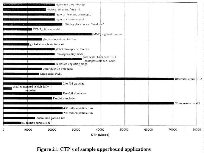
There remains a strong core of applications of national security concern, requiring high levels of computing performance. Figure 21 shows a sampling of specific applications examined for this study. As detailed in later sections of this chapter, these applications continue to demand computing performance well above the current export limits, and in most cases will remain well above the lower bound of controllability for the foreseeable future.
68
Role of Computational Science
Computational science is playing an increasingly important role in research and development in almost every area of inquiry. Where danger exists in the development and testing of prototypes, simulation can reduce the danger. Simulation can support the investigation of phenomena that cannot be observed. Simulation reduces costs by reducing the number of different prototypes that need to be built. Finally, simulation increases the effectiveness of a testing program while reducing the number of actual tests needed.
In some areas, computer simulation is already a tightly integrated part of the development and testing cycle. In other areas, simulation techniques are still being developed and tested. In all areas, simulation techniques will see continued improvement, as better computer hardware becomes available. This will allow experiments that are not possible today due to constraints of memory and/or processors. Better hardware will also support parametric studies, that is, allow the researcher to run a suite of tests varying one or more of the parameters on each run.
69
In some areas. high performance computing directly supports operational needs. Weather forecasting is a clear example of this. Improved hardware leads directly to more accurate global forecasts. Better global forecasts lead to more accurate regional forecasts. The number of regional forecasts that can be developed within operational time constraints is directly dependent on the computing resources available.
Demand for greater resources
Computational science continues to demand greater computing resources. There are three driving factors behind this quest for more computing performance. First, increasing the accuracy, or resolution, of an application generally allows more detail to become apparent in the results. This detail serves as further validation of the simulation results and provides further insight into the process that the simulation is modeling. Second, increasing the scale of a simulation allows a larger problem to be solved. Examples would be increasing the number of molecules involved in a molecular dynamics experiment or studying a full-size submarine complete with all control surfaces traveling in shallow water. Larger problems thus become a path into understanding mechanisms that previously could only be studied through actual experiments, if at all. Finally, moving to models with greater fidelity. Examples here include using full physics rather than reduced physics in nuclear applications and solving the full Navier-Stokes equations in fluid dynamics problems.
All three--increased resolution, increased scale, and improved fidelity--offer the possibility of a quantum leap in understanding a problem domain. Examples include studies of the dynamics among atoms and molecules of an explosive material as the explosive shock wave proceeds, or eddies that form around mid-ocean currents. Ideally, a good simulation matches the results of actual observation, and provides more insight into the problem than experiment alone.
Increased resolution and scale generally require a greater than linear growth in computational resources. For example, a doubling of the resolution requires more than a doubling of computer resources. In a three-dimensional simulation, doubling the resolution requires a doubling of computation in each of three dimensions, a factor of eight times the original. And this example understates the true situation, as a doubling of the resolution often requires changes in the time scale of the computation resulting in further required increases in computing resources.
Memory demands are often the motivation behind a move from a traditional vector platform to a massively parallel platform. The MPP platforms offer an aggregate memory size that grows with the number of processors available. There are currently MPP machines that have one gigabyte of memory per node, with node counts above 200.2 The attraction of such large memory sizes is encouraging researchers to make the effort required (and it is considerable) to move to the parallel world.
_______________________
2 Aeronautical Systems Center (ASC), a DoD Major Shared Resource Center located at Wright-Patterson AFB has a 256 node IBM SP-2 with one gigabyte of memory per node, for a total of 256 gigabytes.
70
Transition from parallel-vector to massively-parallel platforms
Scientific applications in all computational areas are in transition from parallel vector platforms (PVP) to massively parallel platforms (MPP). Hardware developments and the demands--both price and performance--of the commercial marketplace, are driving this transition. These trends have already been discussed in detail in chapter 2. Computational scientists in some application areas made early moves to MPP platforms to gain resources unavailable in the PVP platforms--either main memory space or more processors. However, all areas of computational science are now faced with the need to transition to MPP platforms.
The development of platform independent message-passing systems, such as PVM [2] and p4 [3], supported the first wave of ports from traditional PVP machines to MPP machines. The platform independence helped assure the scientists that their work would survive the vagaries of a marketplace that has seen the demise of a number of MPP manufacturers. The development of the Message Passing Interface [4] standard in 1994 and its wide support among computer manufacturers has accelerated the move to MPP platforms by scientists.
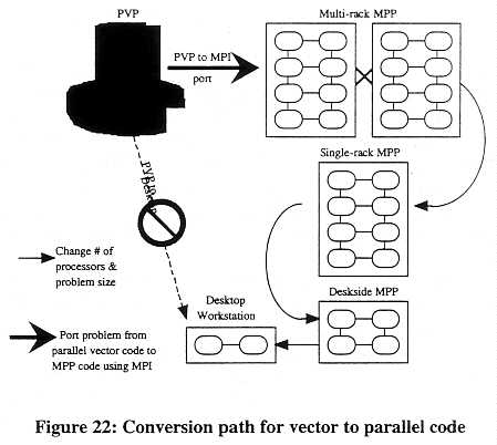
The move to MPI has resulted in applications that can run effectively on a broad range of computing platforms and problem sizes, in contrast to PVP codes that rely heavily on vector operations for efficient execution. Figure 22 illustrates the transitions possible. From a code optimized for vector operations, it is not easy to obtain a code that runs well on a desktop workstation, or any strictly parallel machine. However, once the effort has been made to port the PVP code to the MPP platform using MPI, it is an easy transition to run the same code on smaller
71
or larger MPP systems by simply specifying the number of processors to use. Since all the computer manufacturers provide support for MPI, the code is now portable across an even wider variety of machines.
The smaller systems generally cannot run the same problems as the larger systems due to memory and/or time constraints. However, being able to run the code on smaller systems is a great boon to development. Scientists are able to test their code on the smaller, more accessible, systems. This shortens the development cycle and makes it possible for researchers without direct access to the larger platforms to be involved in the development and verification of new algorithms.
Parallel coding starting to "come naturally"
Production codes are now entering their second generation on parallel platforms in some application areas. Examples include work in the nuclear area, ocean modeling, and particle dynamics. A common characteristic in many of these applications is a very high memory requirement. Starting roughly with the Thinking Machines CM2, parallel machines began offering greater memory sizes than were available on vector machines. This offered the opportunity to run simulations if the researcher was willing to put in the effort to port the code. Now, those researchers are entering second and even third generation revisions of their codes, and have production as well as R & D experience with parallel machines. Thus, there is a growing cadre of researchers for whom parallel codes have become the ordinary way of working.
Parallel platforms used for production work
Large parallel platforms are being used for production work, as well as for research and development. In general, this use is in application areas that were among the earliest to make the move from the vector processors. Examples include nuclear simulations, particle simulations, cryptographic work, and ocean modeling.
Memory size and bandwidth remain bottlenecks.
Many application areas are moving to parallel platforms primarily to gain the increased aggregate memory sizes available on these systems. The memory to CPU bandwidth then becomes a problem on the commodity RISC-based processors used on the parallel systems. Many problems become sensitive to the size of the cache and often require work to optimize the cache performance.
The other side of this argument, however, is the increased memory sizes available on standard workstations. Problems are now being executed on these workstations that were on supercomputer-class systems a few years ago. These problems were often run as single-CPU jobs on the vector machines, as the primary requirement was the memory size. On workstations, they can require long execution times and often require large disk space as well. However, given the wait time for sufficient resources on high-end computers, it can turn out to be quicker to use a
72
workstation. Where multiple workstations are available, parametric studies can be run simultaneously.
Computing Platforms and Scientific Applications
This section provides a brief discussion of key factors that affect the performance of an application on a parallel computer. A great deal of detail has been omitted to make the discussion accessible. Details that affect specific application areas are covered later in this chapter.
Determinants of performance
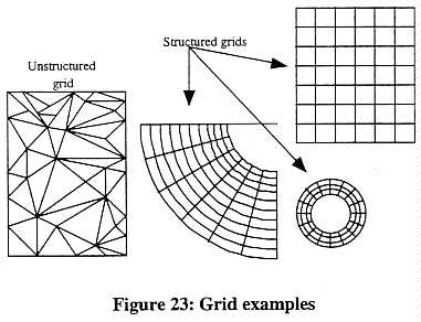
Most scientific applications make use of grids to subdivide the problem space. Grids can be unstructured or structured. Unstructured grids are typically triangular for 2-D problems and tetrahedral for 3-D problems. Finite element (FE) solution techniques are used with unstructured grids. Structured grids are "logically" Cartesian or rectangular in form. Finite difference (FD) or finite volume (FV) solution techniques are used with structured grids. Figure 23 gives some two dimensional examples of solution grids.
In parallel processing, the grids are divided in some fashion across two or more processes, a step known as "domain decomposition." Each process performs the computations on its portion of the grid. At various times during the computation, it is normally necessary for the processes to share data from their portion of the grid with the processes handling the adjacent portions of the grid. When executing on a parallel machine that has multiple processors, each process is typically assigned to one processor. This spreads the computational work over as many processors as are available.
During execution of an application that is spread across multiple processors, each processor will, generally speaking, be in one of three states at a given time:
73
The total execution time (T) of a given processor is the sum of the times spent in each of these three states:
T = Tcomp + Tcomm + Tidle
Tcomp is a function of the number of processes executing on the processor. For each process, Tcomp is further dependent on the grid size, the number of time steps, the number and types of operations executed in each time step, and the time needed to execute an operation. More complex (and realistic) performance models take into account differences in the time needed to execute an operation depending on where data are located (e.g. main memory or secondary storage).
Tcomm is the amount of time the processor spends on exchanging data with other processors. This will be platform dependent, and is dependent on the architecture--shared memory vs. distributed memory.
Tidle is the time a processor spends waiting for data. Generally, this will be while waiting for another processor to complete a task and send the needed data, or merely waiting for requested data to arrive at the CPU.
If execution time is measured from the instant the first processor begins until the last processor ceases activity, then the total execution time for each processor will be the same, although the percentage of time spent in each state is likely to vary.
If only compute time directly advances the state of the computation and the amount of computation necessary for the execution of a particular model and problem size is relatively constant, then performance can best be improved by minimizing the time the processors spend communicating or being idle. The communication requirements strongly depend on the domain decomposition used--how a problem is divided across the multiple processes and how the processes are divided across the machine' s available processors. Different decompositions of the same problem onto the same set of processors can have widely different communication patterns. One goal of problem decomposition is to maximize t'ne amount of computation performed relative to the amount of communication.
Applications and the algorithms they use can differ considerably in how easy it is to find decompositions with good computation-to-communication ratios. So-called "embarrassingly parallel" applications are those that lend themselves to decompositions in which a great deal of computation can be performed with very little communication between processors. In such cases, the execution of one task depends very little, or not at all, on data values generated by other tasks. Often, applications with this characteristic involve solving the same problem repeatedly, with different and independent data sets, or solving a number of different problems concurrently.
74
Shared memory multiprocessor systems.
One broad category of multiprocessors is the shared-memory multi-processor, where all the processors share a common memory. The shared memory allows the processors to read and write from commonly accessible memory locations. Systems in this category include symmetrical multiprocessors (SMP) such as the Silicon Graphics Challenge and PowerChallenge systems, Sun Microsystems' Enterprise 10000, and many others. Cray's traditional vector-pipelined multiprocessors can also be considered part of this broad category, since each processor has equal access to shared main memory.
In the abstract, shared memory systems have no communication costs per se. Accessing the data values of neighboring grid points involves merely reading the appropriate memory locations. Most shared-memory systems built to date have been designed to provide uniform access time to main memory, regardless of memory address, or which processor is making the request.
In practice, the picture is more complex. First, processors must coordinate their actions. A processor cannot access a memory location whose content is determined by another processor until this second processor has completed the calculation and written the new value. Such synchronization points are established by the application. The application must balance the workload of each processor so they arrive at the synchronization points together, or nearly so. Time spent waiting at a synchronization point is time spent not advancing the computation.
Second, most of today's shared-memory machines include caches as part of the memory design. Caches are very fast memory stores of modest size located at or near each processor. They hold data and instruction values that have been recently accessed or, ideally, are likely to be accessed in the immediate future. Caches are included in system design to improve performance by reducing the time needed to access instructions and their operands. They are effective because in many cases the instructions and operands used in the immediate future have a high probability of being those most recently used.3 Caches necessarily involve maintaining duplicate copies of data elements. Maintaining the consistency of all copies among the various processors' caches and main memory is a great system design challenge. Fortunately, managing cache memory is not (explicitly) a concern of the programmer.
The existence of cache memory means that memory access is not uniform. Applications or algorithms with high degrees of data locality (a great deal of computation is done per data element and/or data elements are used exclusively by a single processor) make good use of cache memory. Applications which involve a great deal of sharing of data elements between processors, or little computation per data element are not likely to use cache as effectively and, consequently, have lower overall performance for a given number of computations.
___________________
3 For example, a typical loop involves executing the same operations over and over. After the first iteration, the loop instructions are resident in the cache for subsequent iterations. The data values needed for subsequent iterations are often those located in memory very close to the values used on the first iteration. Modern cache designs include fetch algorithms that will collect data values "near" those specifically collected. Thus, the data for several iterations may be loaded into the cache on the first iteration.
75
Third, when the processors in a shared-memory multiprocessor access memory, they ma~ interfere with each other's efforts. Memory contention can arise in two areas: contention for memory ports and contention for the communications medium linking shared memory with the processors. Memory may be designed to give simultaneous access to a fixed and limited number of requests. Usually, separate requests that involve separate banks of memory and separate memory ports can be serviced simultaneously. If, however, two requests contend for the same port simultaneously, one request must be delayed while the other is being serviced.
A shared communications medium between memory and processors can also be a bottleneck to system performance. internal busses, such as those used in many SMP systems can become saturated when many processors are trying to move data to or from memory simultaneously. Under such circumstances, adding processors to a system may not increase aggregate performance. This is one of the main reasons why maximum configuration SMP's are rarely purchased and used effectively.
Some systems use switched interconnects rather than a shared medium between processors and memory. While more expensive, switched interconnects have the advantage that processors need not contend with each other for access. Contention for memory may still be a problem.
Distributed memory multiprocessor systems.
Distributed memory machines can overcome the problems of scale that shared memory systems suffer. By placing memory with each processor, then providing a means for the processors to communicate over a communications network, very large processor counts can be achieved. The total amount of memory can also be quite large. In principle, there are no limits to the number of processors or the total memory, other than the cost of constructing the system. The SGI Origin2000, Cray T3E, and IBM RS/6000 SP are examples of distributed memory architectures that are closely coupled. Clusters of workstations are distributed memory machines that are loosely coupled.
For distributed memory machines, the communication time, Tcomp, is the amount of time a process spends sending messages to other processes. As with shared memory machines, two processes that need to share data may be on the same or different processors. For a given communication (sending or receiving a message), communication time breaks into two components: latency and transmission time. Latency time--in which various kinds of connection establishment or context switching are performed--is usually independent of the message size. It is dependent in varying degrees on the distance between processors and the communication channel. Transmission time is a function of the communication bandwidth - the amount of data that can be sent each second--and the volume of data in a message. The distinction between closely coupled and loosely coupled machines lies primarily in the latency costs, as explained in chapter 2.
Even for applications that are not embarrassingly parallel, the ratio of computation to communication can sometimes be improved by increasing the granularity of the problem, or the portion of the problem handled by a single processor. T'his phenomenon is known as the surface-to-volume effect. As an illustration, suppose that a problem involved a two-dimensional grid of
76
data points. Updating the value at each point involves obtaining the values of each of the four neighboring points. If a different processor is used to update each grid point. then for one computation, four communications are required to obtain the neighbor's data values. If, however. each processor were responsible for updating an 8 x 8 = 64 grid-point portion of the grid, 64 computations would be needed (one for each grid point), but only 8 x 4 = 32 communications. No communication is involved in accessing data from a neighboring grid point when the data values are stored in the memory of the same processor. Communication occurs only for fetching the data values of grid points lying outside the perimeter of the 64-point grid, since these are located in the memory of other processors. In a two-dimensional grid, the amount of computation is proportional to the number of points in a subgrid (the volume), while the amount of communication is proportional only to the number of points on the perimeter (the surface). Further, the messages often can be batched along an edge. Following the same example, the one processor can request the 8 values for one side of its grid in a single message, and can send its own 8 values on the same edge in one message. The amount of data sent will be the same, requiring the same bandwidth; however, the latency will be reduced since the start-up cost needs to be paid for only one message, not eight.
While increasing the granularity for a fixed-sized problem improves the computation-to-communications ratio, it also reduces the amount of parallelism brought to bear. (The extreme case would be putting the entire problem on a single processor: excellent computation-to-communications ratio, but no parallelism.) For a fixed number of processors, however, the computation-to-communication ratio can be improved by increasing the size of the problem and, correspondingly, the number of grid points handled by a single processor. This assumes, however, that the processor's memory is large enough to hold the data for all the points; the paging overhead associated with virtual memory is likely to decrease performance dramatically.
Numerical Weather Forecasting
Introduction
Weather conditions have always played a vital role in a host of military and civilian activities. The ability to predict in advance the weather conditions in a particular area can provide a substantial competitive advantage to those planning and executing military operations. For this reason, in spite of the obviously beneficial civilian applications, weather forecasting is considered an application of national security significance.
Since the dawn of the computer age, the most advanced computing systems have been brought to bear on computationally demanding weather forecasting problems. Historically, weather forecasters have been among the leading adopters of new supercomputing technology. While this tradition continues to the present, weather forecasters have been challenged by the broadening base of computing platforms that, in principle, can be used in weather forecasting. Besides the well-established vector-pipeline processors, practitioners have other options, including massively parallel and symmetrical multiprocessor systems.
77
Numerical weather forecasting was identified in Building on the Basics as a crucial upper-bound application. This section examines the computational nature of numerical weather forecasting in much greater detail than did the previous study, with the goal of understanding to what degree such applications can be usefully executed on a variety of system architectures, principally vector-pipeline and massively parallel processors. Ultimately, the goal is to understand the degree to which forecasting of a nature useful to military operations can be performed on the uncontrollable computer technology of today and tomorrow.
This section starts by examining the relationship between the computational nature of the application and the major high-performance computer architectures currently available. The next subsection includes a discussion of empirical results obtained from leading forecasting centers in the United States and Europe regarding the use of various platforms to run their atmospheric models. Then we discuss global and regional ocean forecasts and their similarities and differences from atmospheric models. Finally, we conclude with a brief discussion of future trends in numerical weather forecasting and computational platforms, and alternative sources of competitive advantage for U.S. practitioners.
The Computational Nature of Numerical Weather Forecasting
The state of the weather at any given point in time can be defined by describing the atmospheric conditions at each point in the atmosphere. These conditions can be characterized by several variables, including temperature, pressure, density, velocity (in each of three dimensions). Over time, these conditions change. How they change is represented mathematically by a set of partial differential and other equations that describe the fluid dynamic behavior of the atmosphere and other physical processes in effect. The fluid dynamics equations include:
conservation of momentum
conservation of water substance4
conservation of mass
conservation of energy
state (pressure) equation
Equations for physical processes describe such phenomena as radiation, cloud formation, convection, and precipitation. Depending on the scale of the model, additional equations describing localized turbulence (e.g. severe storms) may be used.
Collectively, these equations constitute an atmospheric model. In principle, if the state of the weather at a given time is known, the state of the weather at a future time can be determined by performing a time integration of the atmospheric model based on these initial conditions.
The basic equations and the atmosphere itself are continuous. Like many numerical models of physical phenomena, however, the atmospheric models approximate the actual conditions by
___________________
4 The conservation of water substance equations govern the properties of water in various states: vapor, cloud, rain, hail, snow.
78
using a collection of discrete grid points to represent the atmospheric conditions at a finite number of locations in the atmosphere. For each grid point, values are stored for each of the relevant variables (e.g. temperature, pressure, etc.).
Future weather conditions are determined by applying discrete versions of the model equations repeatedly to the grid points. Each application of the equations updates the variables for each grid point and advances the model one "time step" into the future. If, for example, a single time step were 120 seconds (2 minutes), a 24-hour forecast would require 24 hours/2 minutes = 720 applications (iterations) of the model's equations to each grid point.5
The fluid dynamics of the atmosphere is typically modeled using either a finite difference method, or a spectral transform method. With the finite difference methods, variables at a given grid point are updated with values computed by applying some function to the variables of neighboring grid points. During each time step, the values at each grid point are updated, and the new values are exchanged with neighboring grid points.
The spectral transform methods are global spherical harmonic transforms and offer good resolution for a given amount of computational effort, particularly when a spherical geometry (like the earth) is involved.6 The drawback, however, is that the amount of computation necessary in spectral methods grows more quickly than in finite difference methods as the resolution increases. Practitioners are divided on which method is better.
Numerical weather prediction models carl also vary in the scale of the model, the length of the forecast, the physical phenomena to be modeled, and the degree of resolution desired. The models vary in the number of grid points used (and, in the case of spectral methods, the number of waves considered in the harmonics),7 the number of time-steps taken, and the equations employed.
Current models used in military weather forecasting can be classified as global, mesoscale (regional)8, theater, or battlespace (storm-scale). The domain for these models ranges from the entire planet (Global) to a 1000 x 1000 km region (battlespace). For each of these models, weather can be forecast for a variety of time periods into the future. Typical forecasts today are from I2 hours to 10 days.
_____________________
5 The Naval models described below use time steps of 440s for global models, 120s for regional models, and smaller time steps for each under certain circumstances, such as when there are high atmospheric winds, or when higher resolution is needed for localized conditions. Other models may use different time steps.
6 The basic grid point mesh has a rectangular solid geometry. The spherical geometry of the earth means that if the same number of grid points represents each latitude, the geographic distance between these points is less as you approach the North or South Pole. Such considerations introduce complexities into the finite difference algorithms.
7 The resolution of models using spectral techniques is usually indicated by the convention Tn, where n is the number of harmonics considered. A model designated T42 has a lower resolution than one designated T170. The NOGAPS (Global) model used by Fleet Numerical is designated T159.
8 Mesoscale models typically model a domain with a scale of a few thousand kilometers. Such models are particularly useful for forecasting severe weather events, simulating the regional transport of air pollutants, etc. Mesoscale models are regional models, but the latter term is also used to describe extracts of global models.
79
Models can also be classified as hydrostatic, or non-hydrostatic. Hydrostatic models are designed for use on weather systems in which the horizontal length scale is much greater than the vertical length scale. They assume that accelerations in the vertical direction are small, and consequently are not suitable for grid spacing below 5-10 km. Non-hydrostatic models. on the other hand, do not make this assumption and are often employed in systems that model, for example, thunderstorms or other phenomena on this scale. Current military models that emphasize global and regional forecasts are hydrostatic, but work is being done to develop non-hydrostatic models as well.
The resolution of the model depends on both the physical distance represented by two adjacent grid points, and the length of the time step. A model in which grid points represent physical coordinates 20 km apart will generally give more precise results than one in which grid points offer a resolution of only 100 km. Similarly, shorter time steps are likely to yield better results than longer ones. The greater the resolution, the greater the fidelity of the model. For example, certain kinds of turbulence may be modeled with grid points at 1 km, but not 80 km, resolution. At the same time, however, increasing the number of grid points or decreasing the time step increases the amount of storage and computation needed.
The choice of grid size, resolution, and timestep involves balancing the type of forecast desired against the computational resources available and the time constraints of the forecast. To provide useful predictions, a model must run sufficiently fast that the results are useful (e.g. a 24-hour forecast that takes 24 hours to compute is of no use.) For this reason, there are clear limits to the size of the model that can be run on a given platform in a given time window. On the other hand, there are points beyond which greater resolution is not needed, where practitioners feel a particular model size is sufficient for a desired forecast. For example, the "ultimate" domain size necessary for storm-scale prediction is a 1024 x 1024 x 32 grid [5].
Military Numerical Weather Forecasting
Military Numerical Weather Forecasting Models
Table 11 shows some of the models used by the Fleet Numerical Meteorology and Oceanography Center for military numerical weather prediction, as of the end of 1995 [6]. The global models are currently their principle products. The right-hand column indicates the elapsed time needed to run the model.
80
| Type | Definition | Resolution | Wall Time |
| Global Analysis | MVOI9 | Horizontal: 80 km Vertical: 15 levels |
10 min/run |
| Global Forecast | NOGAPS10 3.4 | Horizontal: 80 km Vertical: 18 levels |
30 min/forecast day |
| Regional 9000 km x 9000 km |
NOGAPS Extracts |
||
| Theater 7000 km x 7000 km |
NORAPS11 6.1 relocatable areas |
Horizontal: 45 km Vertical: 36 levels |
35 min/area |
| Mesoscale 3500 km x 3500 km |
NORAPS 6.1 2 areas
NORAPS 6.1 |
Horizontal: 20 km Vertical: 36levels
Horizontal: 15 km |
60 min/area 75 min/area |
Table 11. Weather prediction models used by Fleet Numerical MOC.
To understand the significance of the wall time figures, it is important to understand the real-time constraints of a center like Fleet Numerical. Weather forecasting is not a one-time computation. Fleet Numerical's many customers require a steady stream of forecasts of varying duration. Given a finite number of CPU hours per day, the CPU time used to generate one forecast may take time away from another. For example, if a global forecast were to take 45 rather than 30 minutes per forecast day, one forecast might start encroaching on the time allocated for the next forecast. Either the number of forecasts, or the duration of each, would have to be reduced. When weather forecasters increase the resolution or the grid size of a particular model but use the same hardware, one forecast run can start cutting into the next run. For example, when the mesoscale model was run to support NATO operations in Bosnia, improving resolution from 20km to 15km doubled the run time. Better resolution would be possible computationally, but impossible operationally on the current hardware. Operational considerations place strong constraints on the types of models that can be run with the available hardware.
_________________
9 Multi-variate Optimum Interpolation. Used to provide the initial conditions for both the global and regional models (NOGAPS and NORAPS), but at different resolutions.
10 Navy Operational Global Atmospheric Prediction System.
11 Navy Operational Regional Atmospheric Prediction System.
81
The Traditional Environment for Military Numerical Weather Forecasting
The current state of military numerical weather forecasting in the United States is a result of a number of current and historical circumstances that may or may not characterize other countries weather forecasting efforts.
In summary, Fleet Numerical operates on very demanding problems in a very demanding environment and is, for good reasons, rather conservative in its use of high-performance computing. The Center is not likely to dramatically change the models, code, or hardware/software platforms it uses until proven alternatives have been developed. Fleet Numerical practitioners make it clear that current models and codes do not (yet) run well on distributed-memory, or non-vector-pipelined systems.12 This is only partly a function of the nature of numerical weather forecasting (discussed in the next section). It is as much, or more, a function of the development and operational environments at Fleet Numerical and the Naval
___________________
12 The Cray vector-pipelined machines reportedly provide a sustained processing rate of 40% of the peak performance on Fleet Numerical codes. For example, the 8-processor C90 has a peak performance of 7.6 Gflops and provides just over 3 Gflops of sustained performance.
82
Research Labs that develop the supporting models. Since the current generation of software tools is inadequate for porting 'dusty deck, legacy" Cray code to massively parallel platforms, the human effort of porting the models would be comparable to developing new models from scratch Furthermore, there is, as described below, little guarantee that the end result would be superior to current practice. The risk to Fleet Numerical operations of moving to dramatically new models and platforms prematurely is considerable. Consequently, those interested in understanding the suitability of non-traditional hardware/software platforms for (military) numerical weather forecasting should consider as well the experience of practitioners at other meteorological centers, who might be less constrained by operational realities and more eager to pioneer innovative approaches.
Computing Platforms and Numerical Weather Forecasting
This section examines the computational characteristics of numerical weather forecasting, with an emphasis on the problems of moving from vector platforms to massively parallel platforms. The first half of the section examines the problem in general. The second half explores a number of specific weather codes and the platform(s) they execute on.
Numerical Weather Forecasting and Parallel Processing
Like many models describing physical phenomena, atmospheric models are highly parallel; however, they are not embarrassingly so. When a model is run, most of the equations are applied in the same way to each of the grid points. In principle, a different processor could be tasked to each grid point. During each time step, each processor would execute the same operations, but on different data. If computation done at one grid point were independent of computation done at another, each processor could proceed without regard for the work being done by another processor. The application would be considered embarrassingly parallel and nearly linear improvements in performance could be gained as the number of processors increases.
However, computation done at one grid point is not, in fact, independent of that done at another. The dependencies between grid points (described below) may require communications between processors as they exchange grid point values. The cost in CPU cycles of carrying out this sharing depends a great deal on the architecture and implementation of the hardware and systems software.
There are three kinds of data dependencies between grid points that complicate the parallel processing of weather forecasting models. First, at the end of each time step, each grid point must exchange values with neighboring grid points. This involves very local communications. How local depends on the algorithm. In higher-order finite difference schemes, the data needed to update a single grid point' s variables are drawn not just from the nearest neighboring grid points, but also from grid points that are two or more grid points away. The amount of communications is subject to the surface/volume phenomenon described earlier.
The spectral methods, an alternative to the finite difference methods, often involve transforms (between physical, Fourier, and spectral space) that have non-local communications patterns.
83
Second, global operations, such as computing the total mass of the atmosphere. are executed periodically. Good parallel algorithms exist for such computations.
Third, there are physical processes (e.g. precipitation, radiation, or the creation of a cloud) which are simulated using numerical methods that draw on data values from a number of different grid points. The communications costs can be considerable. The total physics component of an atmospheric model can involve two dozen transfers or more of data per grid point per time step. However, the grid points involved in such a simulation usually lie along the same vertical column. Assigning grid points to processors such that all grid points in the same vertical column are assigned to the same processor typically reduces communications costs.
In many models, a so-called semi-Lagrangian transport (SLT) method is used to update the moisture field at grid points. This method computes the moisture content at a grid point (the "arrival point") by tracking the trajectory of a particle arriving at this grid point back to its point of origin in the current time step ("departure point"). The moisture field of the departure point is used in updating the moisture field at the arrival point. This computation can involve significant communications overhead if different processors are handling the arrival and departure points.
Finally, overall performance of a model is strongly affected by load-balancing issues related to the physics processes. For example, radiation computations are performed only for grid points that are in sunlight [7]. The computational load can be distributed more evenly among processors, but usually at the cost of great communications overhead.
Performance of Computing Platforms: Empirical Results
Since the first weather forecasting models were run on the ENIAC, meteorologists have consistently been among the first practitioners to make effective use of new generations of supercomputers. The IBM 360/195, the Cray 1, the Cyber 205, the Cray YMP and Cray C90 have all been important machines for weather forecasting [8]. In 1967, weather codes were adapted for the SOLOMON II parallel computer, but the amount of effort devoted to adapting weather models and algorithms to parallel systems, both shared-memory and distributed memory, has grown dramatically only in the 1990s, as parallel systems have entered the mainstream of high-performance computing.
Meteorologists at leading research institutes and centers throughout the world have done a great deal of work in adapting weather codes for parallel platforms and obtaining empirical results. These efforts include:
84
The weather and climate forecasting problem domain currently embraces a significant number of different models, algorithms, implementations, and hardware platforms that make it difficult to provide highly detailed performance comparisons. At the same time, the general conclusions are remarkably consistent:
Ocean Forecasts
Global ocean forecasts have two purposes. The first is to predict the ocean currents. An ocean current has eddies and temperature variations that occur within and around the current flow. The temperature differences become important in submarine and anti-submarine warfare. The side that knows where the current is and is not can both hide its submarines more effectively and improve the chances of detecting other submarines. Ocean currents also become important in
85
ship routing decisions, both for lowering fuel costs and shortening transit times. This latter application of ocean modeling has both civilian and military uses.
The second purpose of an ocean forecast is to provide the sea surface temperature input used as one of the major inputs to the atmospheric forecasts. An ocean model that can provide more accurate surface temperatures will enable an atmospheric forecast with improved accuracy. To date, however, attempts to directly couple the two models to provide this input have not been successful. It is believed this is primarily due to the ocean models using a coarser resolution than the atmospheric forecasts.
Ocean models take as their input the winds, sea state information (especially wave height), and sea surface temperature [16]. An atmospheric forecast can provide heat, moisture, and surface fluxing as inputs to the ocean model. The heat input determines sea surface temperature and the surface fluxing affects wave creation. Wind information can be taken in part from observation, but primarily comes from the atmospheric forecast. The ocean model requires averaging information about the winds; that is, the ocean model needs the average of the winds over a period of days rather than the specific wind speeds at a particular instant. Current sea surface temperature and wave height information is also obtained from satellite data. The wave height information is used in part to determine average wind speeds. The satellite data comes from the GEOSAT series of satellites from the U.S. Both Japan and France have similar satellites. Altimeter equipped satellites can provide additional data about the currents. For example, a cross-section of the Gulf Stream will show variations in ocean height of up to a meter as you move across the current. Current satellite altimeters can measure differences in height of a few centimeters.
Ocean models are complicated by the need to accurately predict the behavior below the surface, yet there is very little data about the current state of the ocean below the surface. A11 of the observation-based data is about the surface or near surface. Thus, a good climatological model is essential to get the deep ocean correct. Statistical inference is used to move from the surface to the deep ocean based on ocean models. There are now about 15 years worth of ocean model data to draw upon.
Ocean models are characterized by the size of the cells used to horizontally divide the ocean. Thus, a 1/4 degree ocean model uses cells that are 1/4 degree longitude by 1/4 degree latitude on each side, yielding a resolution of about 25 km on a side. This is the current model used at Fleet Numerical for their daily ocean current forecasts and run on their 12 processor C90. This model simply examines the first 50 m of water depth, looking at temperature variations due to wind stirring and heat at the surface. This is a global model covering all the world's oceans except the Arctic Ocean. Regional current models are used for finer granularity in areas of particular interest, such as smaller seas, gulfs, and coastal areas. These models run at various finer resolutions that depend on the nature of the region covered and its operational importance. The global model serves as the principle input to the regional models.
This operational global ocean model is too coarse to provide useful current information. In addition, it does not provide sufficient resolution to be useful as input to the atmospheric model.
86
The limitation is one of time--Fleet Numerical allocates one hour of C90 time for each ocean forecast. A secondary limitation of the C90 is insufficient memory
Researchers at the Naval Oceanographic Office (NAVO) at the Stennis Space Center are developing more accurate models. In part, these are awaiting procurement decisions at Fleet Numerical However, even these models will not be able to produce sufficient accuracy within the one hour time constraint to model the ocean currents.
A 1/32 degree (3 km resolution) ocean model is the goal This will provide good coverage and detail in the open ocean, and provide much better input to the regional and coastal models. This goal is still some years out. The current roadmap for Fleet Numerical with regard to ocean current models is shown in Table 12.
| Date | Cell Resolution |
Coverage | |
| present | 1/4 degree | 25 km | global |
| 2001 | 1/8 degree
1/16 degree 1/32 degree |
12-13 km
7 km 3 km |
global
Pacific Atlantic |
| -2007 | 1/32 | 3 km | global |
Table 12: Global ocean model projected deployment [16]
The vertical resolution in these models is six vertical layers. The size of a vertical layer depends on the density of the water, not its depth. Using fixed-height layers would increase the vertical requirement to 30 or more layers to gain the same results. The depth of the same density will change by several hundreds of meters as the grid crosses a current or eddy.
Researchers at NAVO are working with Fortran and MPI. The code gains portability by using MPI. In what has become a standard technique across disciplines, the communication code is concentrated within a few routines. This makes it possible to optimize the code for a particular platform by easily substituting the calls for a proprietary communication library, such as Cray's SHMEM.
It takes five to six years to move a model from an R & D tool to a production tool. In addition to the time needed to develop the improved models, the model must be verified. The verification stage requires leading edge computing and significant chunks of time. The model is verified using "hindcasts"--executions of the model using historic input data and comparing the output with known currents from that time frame. For example, NAVO tested a 1/16 degree (7 km) global ocean model in May-June 1997 on a 256-node T3E-900 (91,000 Mtops). It required 132,000 node hours, about 590 wall clock hours.13 Such tests not only establish the validity of the new model, they improve the previous model. By comparing the results of two models at
___________________
13 224-nodes were used as compute nodes. The remaining 32 nodes were used for I/O.
87
different resolutions, researchers are often able to make improvements on the lower resolution model. Thus, the research not only works toward new production models for the future, but also improves today's production codes.
Ocean models made the transition to MPP platforms much earlier than the atmospheric models. "Oceanographic codes, though less likely to have operational time constraints, are notorious for requiring huge amounts of both memory and processor time" [17]. Starting with the Thinking Machines CM-5, ocean codes on MPP platforms were able to outperform the Cray PVP machines. For example, the performance of an ocean model on a 256-node CM-5 ( 10,457 Mtops) was equivalent to that achieved on a 16-node C90 (21,125 Mtops) [16]. Ocean codes are also more intrinsically scalable than atmospheric codes. There is not as much need to communicate values during execution, and it is easier to overlap the communication and computation parts of the code. Sawdey et al [17], for example, have developed a two-tier code, SC-MICOM, that uses concurrent threads and shared memory within an SMP box. When multiple SMP boxes are available, a thread on each box handles communication to the other SMP boxes. Each box computes a rectangular subset of the overall grid. The cells on the outside edges of the rectangular subset are computed first, then handed to the communication thread. While the communication is in progress, the remaining cells inside the rectangular subset are computed. This code has been tested on an SGI Power Challenge Array using four machines with four CPUs each ( 1686 Mtops each), and on a 32-node Origin2000 ( 11,768 Mtops) where each pair of processors was treated as an SMP.
The dominant machine in ocean modeling today is the Cray T3E. It is allowing a doubling of the resolution over earlier machines. Several systems are installed around the world with 200+ nodes for weather work, including a 696-node T3E-900 (228,476 Mtops) at the United Kingdom Meteorological Office. These systems are allowing research (and some production work) on ocean models to advance to higher resolutions.
Modeling coastal waters and littoral seas
Modeling ocean currents and wave patterns along coasts and within seas and bays is an application area with both civilian and military interests. These include:
88
The military time constraints are hard These regional models are used as forecasts for military operations. Civilian work. on the other hand, does not typically have real time constraints. The more common model for civilian use is a long-term, months to years, model. This is used for beach erosion studies, harbor breakwater design, etc.
Fleet Numerical is not able to run coastal and littoral models for all areas of the world due to limits on computer resources. Currently, about six regional models are run each day at resolutions greater than the global ocean model. These are chosen with current operational needs and potential threats in mind. They include areas such as the Persian Gulf, the Gulf of Mexico, the Caribbean, and the South China Sea.
It is possible to execute a regional model on fairly short notice for a new area. For example, the Taiwan Straits regional model was brought up fairly quickly during the Chinese naval missile exercises. However, better regional models can be produced when the model is run frequently. This allows the researchers to make adjustments in the model based on actual observations over time. Thus, the Persian Gulf model that is executed now is much better than the model that was initially brought up during the Persian Gulf Crisis [16].
Coastal wave and current models are dependent on a number of inputs:
The Spectral Wave Prediction System (SWAPS) uses nested components. The first component is the deep-water wave-action model. This provides the input to the shallow-water wave action model, for water 20m or less in depth. Finally, when needed, the harbor response model and/or the surf model are used to provide high resolution in these restricted areas. The wave action model Is limited by the accuracy of the atmospheric model [18]. This layered model is typical of the approach used in the regional models. 48 hour forecasts are the norm at Fleet Numerical, though, five day forecasts are possible. The limitation is the compute time available. Five day forecasts can be run when required.
While 3 km resolution is the goal for ocean models, this is only marginal for coastal work. A few years ago, it was thought that a 1 km resolution would be a reasonable target. Now, the goal is down to as low as 100 m. The accuracy desired is dependent on the nature of the water in the region. For example, a large, fresh water river flowing into a basin will cause a fresh-water plume. Both the flow of the fresh water and the differing density of fresh and salt water have to be handled correctly by the regional model [16].
An approach that combines the regional models into the global ocean model would be preferred. This would remove the coupling that is now required, and make the regional models easier to
89
implement. However. this will not be feasible for at least five more years. A more accurate global ocean model is needed first. Then, regional models can be folded into the global model as computing resources become available. One major difference in the deep ocean and shallow ocean models is the method of dividing up the vertical layers in the model. The deep ocean model uses six layers whose size is determined by the density of the water, not its depth. Over a continental shelf and on into shallow waters, a fixed-depth set of layers is used. Thus, both the method of determining the layer depth, and the number of layers, is different in the two models. Having both the global ocean model and the regional model in the same code would make the zoning in the vertical layers easier to solve than the present uncoupled approach.
The Navy is working on new ways of delivering regional forecasts to deployed forces. One approach is to continue to compute the regional forecasts at Fleet Numerical or at the Naval oceanographic office (NAVOCEANO), and send the results to those ships that need it. The other alternative is to place computing resources onboard ship to allow them to compute the regional forecast. The onboard ship solution has two principle drawbacks. First, the ship will need input from the global and regional atmospheric forecasts and the global ocean forecast to run the regional model. Sending this data to the ship may well exceed the bandwidth needed to send the completed regional forecast. Second, there would be a compatibility problem with deployed computers that were of various technology generations. Fleet Numerical is looking into options for allowing deployed forces greater flexibility in accessing the regional forecasts when they need it. Among the options are web-based tools for accessing the forecasts, and databases onboard ships that contain the local geographic details in a format such that the regional model can be easily displayed on top of the geographic data [16].
Weather Performance Summary
Figure 24 shows the CTP requirements for weather applications studied in this report. Table 13 shows a summary of the performance characteristics of the weather applications described in this report sorted first by the year and then by the CTP required. It should be noted that some applications appear more than once on the chart and table at different CTPs. This is particularly true of Fleet Numerical's global atmospheric forecast. As Fleet Numerical has upgraded its Cray C90 from 8 to 12 to (soon) 16 processors, it has been able to run a better forecast within the same time constraints. Thus, the increase in CTP does not give a longer-range forecast, but provides a 10-day forecast which has greater accuracy over the 10-day period.
90

91
| Machine | Year | CTP | Time | Problem | Problem size |
| Cray C98 | 1994 | 10625 | -5 hrs | Global atmospheric forecast, Fleet Numerical operational run [19] |
480 x 240 grid; 18 vertical layers |
| Cray C90/1 | 1995 | 1437 | CCM2, Community Climate Model, T42 [9] | 128 x 64 transform grid, 4.2 Gflops |
|
| Cray T3D/64 | 1995 | 6332 | CCM2, Community Climate Model, T42 [9] | 128 x 64 transform grid, 608 Mflops |
|
| IBM SP-2/128 | 1995 | 14200 | PCCM2, Parallel CCM2, T42 [7] | 128 x 64 transform grid, 2.2 Gflops |
|
| IBM SP-2/160 | 1995 | 15796 | AGCM, Atmospheric General Circulation Model [12] |
144 x 88 grid points, 9 vertical levels, 2.2 Gflops |
|
| Cray T3D/256 | 1995 | 17503 | Global weather forecasting model, National Meteorological Center, T170 [11] |
32 vertical levels, 190 x 380 grid points, 6.1 Gflops |
|
| Cray C916 | 1995 | 21125 | CCM2, Community Climate Model, T170 [9] |
512 x 256 transform grid, 2.4 Gbytes memory, 53. Gflops |
|
| Cray C916 | 1995 | 21125 | IFS, Integrated Forecasting System, T213 [10] |
640 grid points/latitude, 134,028 points/horizontal layer, 31 vertical layers |
|
| Cray C916 | 1995 | 21125 | ARPS, Advanced Regional Prediction System, v 3.1 [5] |
64 x 64 x 32, 6 Gflops | |
| Paragon 1024 | 1995 | 24520 | PCCM2, Parallel CCM2, T42 [7] | 128 x 64 transform grid, 2.2 Gflops |
|
| Cray T3D/400 | 1995 | 25881 | IFS, Integrated Forecasting System, T213 [10] |
640 grid points/latitude, 134,028 points/horizontal layer, 31 vertical layers |
|
| Cray T3D/256 | 1996 | 17503 | 105 min | ARPS, Advanced Regional Prediction System, v 4.0, fine scale forecast [14] |
96 x 96 cells, 288 x 288 km, 7 hr forecast |
| Cray C916 | 1996 | 21125 | 45 min | ARPS, Advanced Regional Prediction System, v 4.0, coarse scale forecast [14] |
96 x 96 cells, 864 x 864 km, 7 hr forecast |
| Origin2000/32 | 1997 | 11768 | SC-MICOM, global ocean forecast, two-tier communication pattern [17] |
||
| Cray C912 | 1997 | 15875 | ~5 hrs | Global atmospheric forecast, Fleet Numerical operational run [19] |
480 x 240 grid; 24 vertical layers |
| Cray C912 | 1997 | 15875 | 1 hr | Global atmospheric forecast, Fleet Numerical operational run [16] |
1/4 degree, 25 km resolution |
| Cray T3E- 900/256 |
1997 | 91035 | 590 hrs | Global ocean model "hindcast" [16] | 1/16 degree, 7 km resolution |
| Cray C916 | 1998 | 21125 | ~5hrs | Global atmospheric forecast, Fleet Numerical operational run [19] |
480 x 240 grid; 30 vertical layers |
Table 13: Weather applications
92
The Changing Environment for Numerical Weather Forecasting
Future Forecasting Requirements
In the next five years, there are likely to be significant changes in the forecasting models used. and the types and frequency of the forecasts delivered. The following are some of the key anticipated changes:
Coupling of Oceanographic and Meteorological Models (COAMPS) and development of better littoral models. Currently, meteorological forecasts are made with minimal consideration of the changing conditions in the oceans. Oceans clearly have a strong impact on weather, but in the current operational environment, the computing resources do not permit a close coupling. The COAMPS models will be particularly important for theater, mesoscale, and battlespace forecasting which are likely to be focused on littoral areas in which the interplay of land, air, and ocean creates particularly complicated (and important) weather patterns. Current estimates are that such computations will require a Teraflop of sustained computational performance and 640 Gbytes of memory.
Shorter intervals between runs. Currently, the models used by Fleet Numerical are being run between one and eight times per day. In the future, customers will want hourly updates on forecasts. This requirement places demands on much more than the computational engine. The amount of time needed to run the model is just one component of the time needed to get the forecast in the hands of those in the field who will make decisions based on the forecast. At present, it takes several times longer to get the initial conditions data from the field and disseminate the final forecast than it does to run the model itself.
Greater resolution in the grids. In the next 5-6 years, Fleet Numerical practitioners anticipate that the resolution of the models used will improve by a factor of two, or more. Table 14 shows these changes. Some of the current customers view resolutions of less than 1 km as a future goal. Weather forecasting with this resolution is necessary for forecasting highly local conditions, such as the difference in weather between neighboring mountain peaks or valleys. Such forecasting is closely related to the next requirement of the future:
Emphasis on forecasting weather that can be sensed. As battlespace forecasting becomes practical, the ability to predict weather phenomena that will impact the movement of troops and equipment, placement of weapons, and overall visibility will be important sources of military advantage. Forecasts will be designed to predict not only natural weather phenomena such as fog, but also smoke, biological dispersion, oil dispersion, etc. These forecasts have obvious civilian uses as well.
Ensemble Forecast System. An Ensemble Forecast System (EFS) using NOGAPS has been included in the operational run at Fleet Numerical. The purpose of EFS is both to extend the useful range of numerical forecasts and to provide guidance regarding their reliability. The Fleet Numerical ensemble currently consists of eight members, each a ten-day forecast. A simple average of the eight ensemble members extends the skill of the medium range forecast by 12 to 24 hours. Of greater potential benefit to field forecasters are products that help delineate forecast
93
uncertainty. Another alternate method is to make simple average ensemble forecasts (SAEF) of several Weather Centers with different analyses and models. Both of these systems attempt to evaluate the effect of Chaos theory on weather forecasting by using many different events to determine the probability distributions of the weather in the future.
| Model Type | Grid Resolution: 1995 | Grid Resolution: 2001 (expected) |
| Global Analysis | Horizontal: 80 km Vertical: 15 levels |
Horizontal: 40 km Vertical: (as required) |
| Global Forecast | Horizontal: 80 km Vertical: 18 levels |
Horizontal: 50 km Vertical: 36 levels |
| Regional 9000 km x 9000 km |
Same as Global Forecast | Same as Global Forecast |
| Theater 7000 km x 7000 km |
Horizontal: 45 km Vertical: 36 levels |
Horizontal: 18 km Vertical: 50 levels |
| Mesoscale 3500 km x 3500 km |
Horizontal: 15 km Vertical: 36 levels
Horizontal: 20km |
Horizontal: 6 km Vertical: 50 levels |
| Battlespace 1000 km x 1000 km |
N/A | Horizontal: 2 km Vertical: 50 levels |
Table 14 Current and projected resolution of weather forecasting models
used by FNMOC.
Future Computing Platforms
Fleet Numerical is currently in a procurement cycle. Their future computing platforms are likely to include massively parallel systems. The migration from the current vector-pipelined machines to the distributed memory platforms is likely to require a huge effort by the Naval Research Labs and Fleet Numerical practitioners to convert not only their codes, but also their solutions and basic approaches to the problem. Gregory Pfister has the following comment about the difficulty of converting from a shared-memory environment to a distributed memory one:
This is not like the bad old days, when everybody wrote programs in assembler language and was locked into a particular manufacturer's instruction set and operating system. It's very much worse.It's not a matter of translating a program, algorithms intact, from one language or system to another; instead, the entire approach to the problem must often be
94
rethought from the requirements on up, including new algorithms. Traditional high-level languages and Open Systems standards do not help [20].
A great deal of effort continues to be made by researchers at the Naval Research Laboratories and elsewhere to adapt current codes to parallel platforms and develop new models less grounded in the world of vector-pipelined architectures. There is little doubt that parallel platforms will play increasingly central roles in numerical weather forecasting. What remains to be seen is how well current and future parallel architectures will perform relative to the vector-pipelined systems.
Currently, work is in progress on porting the NOGAPS global forecast model at Naval Research Laboratory - Monterrey for use as a benchmark in the procurement process. The code is being tested on several platforms including the T3E, SP-2 and Origin2000. The benchmark will be ready by spring 1998 for use in procurement decisions. There are problems with load balancing in the~parallel version. For example, the Sun is shining on half the planet (model) and not the other half. The half in sunshine requires more computation. Using smarter load balancing can solve this. One method employed is latitude ring interleaving to provide a balance of sunshine and dark latitude bands to one processor.
Microprocessor hardware is likely to continue its breathtaking rate of advance through the end of the century. The prevalence of systems based on commercial microprocessors is likely to result in steady improvements in the compilers and software development tools for these platforms. These developments are likely to increase the sustained performance as a percentage of peak performance of the massively parallel systems.
Computational Fluid Dynamics
Computational Fluid Dynamics (CFD) applications span a wide range of air and liquid fluid flows. Application areas studied for this report include aerodynamics for aircraft and parachutes, and submarine movement through the water. The basic CFD equations are the same for all these applications. The differences lie in specifics of the computation and include such factors as boundary conditions, fluid compressibility, and the stiffness or flexibility of solid components (wings, parafoils, engines, etc.) within the fluid. The resolution used in an application is dependent on the degree of turbulence present in the fluid flow, size of the object(s) within the fluid, time scale of the simulation and the computational resources available.
We begin with a description of CFD in aerodynamics, specifically airplane design. Much of the general description of CFD applies to all the application areas; thus, subsequent sections describe only the differences from the aerodynamic section.
CFD in Aerodynamics
The Navier-Stokes (N-S) equations are a set of partial differential equations that govern aerodynamic flow fields. Closed-form solutions of these equations have only been obtained for a few simple cases due to their complex form.
Numerical techniques promise solutions to the N-S equations; however, the computer resources necessary still exceed those available. Current computing systems do not provide sufficient
95
power to resolve the wide range of length scales active in high-Reynolds-number turbulent flows.14 Thus, all simulations involve solution of approximations to the Navier-Stokes equations [2 l]. The ability to resolve both small and large turbulence in the fluid flow separates the simple solutions from the complex solutions.
Solution techniques
Ballhaus identifies four stages of approximation in order of evolution and complexity leading to a full Navier-Stokes solution [21]:
| Stage | Approximation | Capability | Grid | Compute factor |
| I | linearized inviscid | subsonic/supersonic pressure loads vortex drag |
3 x 10³ | 1 |
| II | nonlinear inviscid | Above plus: transonic pressure loads wave drags |
105 | 10 |
| III | Reynolds averaged Navier-Stokes |
Above plus: separation/reattachment stall/buffet/flutter total drag |
107 | 300 |
| IV | large eddy simulation |
Above plus: turbulence structure aerodynamic noise |
109 | 30,000 |
| full Navier-Stokes | Above plus: laminar/turbulent transition turbulence dissipation |
1012 to 1015 | 3 x 10⁷ to 3 x 10¹⁰ |
Table 15: Approximation states in CFD solutions
There are 60 partial-derivative terms in the full Navier-Stokes equations when expressed in three dimensions. Stage I uses only three terms, all linear. This allows computations across complex geometries to be treated fairly simply.
Subsequent stages use progressively more of the N-S equations. Finite-difference approximations are used and require that the entire flow field be divided into a large number of small grid cells. In general, the number of grid cells increases with the size of the objects in the flow field, and with the detail needed to simulate such features as turbulence.
In aircraft design, the stage I approach can supply data about an aircraft in steady flight at either subsonic or supersonic speeds. Stage II allows study of an aircraft changing speeds, particularly crossing the sound barrier. It also supports studies of maneuvering aircraft, provided the
_______________________
14 The Reynolds number provides a quantitative measure of the degree of turbulence in the model. The higher the Reynolds number, the more accurately turbulence can be represented by the model.
96
maneuvers are not too extreme. Thus, an aircraft making a normal turn, climb, and/or descent can be modeled at this stage. A jet fighter making extreme maneuvers, however, requires the addition of the viscous terms of the N-S equations. Stage III can provide this level. It uses all the N-S equations, but in a time-averaged approach. The time-averaged turbulent transport requires a suitable model for turbulence, and no one model is appropriate for all applications. Thus, this is an area of continuing research.
Simulating viscous flow complete with turbulence requires another large step up the computational ladder. Hatay et al [22] report the development of a production CFD code that does direct numerical simulation (DNS) that includes turbulent flow. DNS is used to develop and evaluate turbulence models used with lower stage computations. The code is fully explicit; each cell requires information only from neighboring cells, reducing the communication costs. Hatay et al give results for both NEC SX4 and Cray C90 parallel machines. The code has also been ported to the T3D/E and SP-2 MPP platforms. The code illustrates some of the difficulties with moving CFD applications to parallel platforms. Parallel platforms offer the promise of more memory capacity, necessary to solve usefully large problems. The first task was to run the code on a single processor, but make use of all the memory available on the machine. Then, considerable effort is required to get the communication/computation ratio low enough to achieve useful speedup over more than a few processors. Finally, the code was ported to the distributed memory platforms.
Aircraft design
Building on the Basics [1] established that aircraft design, even for military aircraft, generally falls at or below the threshold of uncontrollability. This has not changed since the 1995 study. Two things have occurred in the past two years, both continuations of trends that stretch back to the early 1990's. First, aircraft design is moving to what can be termed "whole plane" simulations. This refers to the three-dimensional simulation of an entire aircraft, including all control surfaces, engine inlets/outlets, and even embedded simulations of the engines. Within engine development, this same principle is evident in moves to develop high fidelity simulations of each engine component and combine them into a single run. While such whole plane and whole engine simulations are still in development, significant progress has been made.
Second, aircraft codes are moving to parallel platforms from vector platforms. This transition has lagged behind what has been done in other application areas. This is largely due to the poor scalability of the applications used in aerodynamics, and to the memory bandwidth and memory size requirements of the applications. A secondary consideration is the need to validate a code before industry is willing to use it.
Whole plane and whole engine designs
Historically, aircraft designers have used numerical simulation to supplement wind tunnel testing. The numerical simulations support more efficient use of expensive wind tunnel time. In turn, this combination has enabled designers to reduce the number of prototypes that need to be built and tested when designing new airframes and engines. This trend continues today. The main
97
difference now from a few years ago lies in the scale of the numerical simulations. Before, designers would study in detail individual components of an aircraft or an engine, for example, a wing, the tail, a propeller, an engine fan. Today, the goal is to model combinations of these elements, leading to the goal to model the entire aircraft, the entire engine, and simulations that have both the aircraft and its engines in the same model. Such models will not replace wind tunnel tests, nor the construction and testing of prototypes. Instead, they will again increase the effectiveness of each wind tunnel test and further reduce the number of tests required. The end result will be a prototype with a greater chance of success delivered in less time.
To date, whole plane simulations typically take advantage of symmetry to model only one half or one quarter of the aircraft, for example. Where full 3-D simulations are run, they do not take into account the full Navier-Stokes equations. In particular, the turbulence fields are not simulated. Thus, whole aircraft simulations are at Stage II or at best a simplified version of Stage III.
Efforts are underway to solve the integration problems that will arise from combining CFD and structures methods. This work will model the interactions between the structure and the fluid flow. For example, the fluid flow may cause a structure to vibrate or move in some way. Such movement will cause changes in the fluid flow. To accomplish this integration, grid generation needs to be improved since both disciplines use slightly different grids. Additionally, the differences in time scales between structural response and the fluid flows must be addressed.
NASA and aeronautics and engine manufacturers are collaborating on research projects toward this goal. One example from the aeronautics side is a 3-year cooperative research agreement (CRA) recently ended that included IBM, several aeronautics firms, universities and two NASA research centers [23]. Researchers at Boeing used the resources of the NASA Metacenter [24], two IBM SP-2 installations, to work on tiltrotor design: 160-nodes (16,706 Mtops) at Ames and 48-nodes (6500 Mtops) at Langley. The heart of the rotor program is Boeing's comprehensive rotor analysis code. This uses coupled aerodynamics and mechanical dynamics of a rotor. The code incorporates a number of models of different effects associated with helicopter rotor blades and jet engine fan blades. Several of these models were ported to the SP-2 during the study. Improvements are summarized in Table 16.
| Code | Performance Result |
| wake calculation, including rotor performance, vibration, and noise |
previous time: 80 hours current time: 2 to 4 hours |
| coupled codes: rotor motion and deflections rotor CFD analysis |
linear speedup on up to 32 processors |
Table 16: Results of improvements to tiltrotor simulation
The improvement from 80 hours to 2 to 4 hours in run time allows designers to run parametric studies that change only one or two variables on each run. Such studies provide a much more comprehensive understanding of the problem.
98
in another example. the Computing and Interdisciplinary System Office at NASA Lewis Research Center is leading a project that includes jet engine companies to develop a numerical wind tunnel for air breathing propulsion systems.15 The goals are to improve product performance and reduce product development time and cost through improved engine simulations. The work is an outgrowth and extension of the Numerical Propulsion System Simulation project [25]. Sub-goals include improved simulations for the individual engine components, and interdisciplinary studies combining CFD with structures. A major thrust throughout the project has been the development of parallel codes for a variety of platforms, either by porting vector codes or through development of new codes. Other software projects include work on mesh generation codes to support coupling CFD codes with structures codes, the development an engine geometry database, and the use of high speed satellite and land lines for remote operation of engine simulations.
One specific result of this NASA effort is the ENG10 project [26]. ENG10 is an axi-symmetric, complete engine CFD code that models the airflow within and around the jet engine using a Runge-Kutta solution technique. It has been ported from a single-processor version optimized for a vector platform to a parallel version that executes on an SP-2, a T3D, and a cluster of workstations. Considerable effort has been put into optimizing the code, in particular in handling the data layout and communication patterns. The result is a code that shows a speedup of 6.2 on eight processors in a cluster using an ATM network. Further work with this code is focusing on incorporating results from other engine component codes to improve the accuracy of the simulation. A database developed by General Electric Aircraft Engines is being used to provide input from a variety of engine components to ENG10 [27].
Move from vector to parallel systems
Memory bandwidth continues to be the primary deterrent to porting CFD codes to parallel platforms. This has also been the deterrent in the past to running useable codes on smaller platforms in general. The workstations of a few years ago did not have either the raw memory capacity or the memory-CPU bandwidth. This has changed in the last few years with the decline in the cost of memory; although, bandwidth problems remain. Most CFD codes on vector platforms run in single-processor mode, since memory size is the main requirement for the application.
For the commodity-based processors used on current MPP platforms and workstations, the bandwidth problem is a function of the cache performance and main memory performance. CFD codes have a high ratio of data fetches to floating point operations that can easily stress the cache- and memory-management hardware. NUMA architectures compound this difficulty. Historically, CFD codes were run on Cray platforms in single-processor mode, as the primary requirement was access to a large memory system. It was not generally worth modifying the code for parallel operation on the vector machines.
_____________________
15 http://www.lerc.nasa.gov/WWW/CISO/
99
Even before considering issues of parallelism, a CFD code must be revised to handle the differences in memory between the vector shared-memory model and the parallel distributed-memory model. The layout of data for a vector processor is based on appropriate memory strides. The data layout for cache-based systems requires spatial and temporal locality of data. This forces the use of zero- or unit-stride memory arrangements, so a cache line brought from memory will contain not only the currently needed value, but value(s) for the next iteration as well [28]. Once the data issues are resolved, the code can be extended to take advantage of additional processors.
In addition to the memory-related difficulties, larger CFD problems, when ported to parallel platforms, have the following characteristics:
Two examples to illustrate the difficulty in porting CFD codes to parallel platforms come from work sponsored by NASA Ames, where an Origin2000 system was installed in early summer, 1997. The first is a port of ARC3D [29]. The port involved a version of ARC3D that is a simple 3D transient Euler variant on a rectilinear grid. This code has been very inefficient in the past on cache-based systems. The initial port from the C90 to the Origin2000 was easily completed involving only the proper setting of compiler flags to meet the requirement for 64-bit precision. However, optimizing the code then took two months and involved re-writing five major routines, about 1000 lines of code. By comparison, the second example of a port of CFL3D was done without special optimization [30]. CFL3D uses a finite volume approach to solve time-dependent thin-layer Navier-Stokes equations in three dimensions. Table 17 shows the results of these two ports.
| Code | Processors | CTP | Speedup (% of linear) | Mflops (% of peak) |
| ARC3D | 64 | 23,488 | 48.93 (76%) | 98.6 (25%) |
| CFL3D | 12 | 4,835 | 12.3 (103%)16 | 39.7 (10%) |
Table 17: Results of porting two CFD applications from vector to parallel
The interesting comparison is the percent of peak achieved in the two cases. Such percentages are typical of codes ported from vector to parallel platforms. 50% of peak is possible for well-vectorized code on a Cray vector system. The results here of 10% to 25% are more typical of the parallel platforms, and representative of the results when effort is applied to optimize a code for an MPP platform.
________________________
16 The slightly super-linear speedup for 12 processors is believed to be an anomaly associated with the memory layout on the Origin2000. The speedup for fewer processors was near- or sub-linear.
100
Military vs civilian design
Military design differs from civilian in its computational requirements primarily in the need to run simulations that push the envelope of the performance of the aircraft. This requires more computational runs, rather than significantly different types of runs. Components of military aircraft and engines have to perform in a greater range of flight attitudes, altitudes, and speeds than do civilian aircraft. The result is the need for a greater number of parametric runs. Such demands can be met by providing more computing capability; that is, more computers rather than necessarily more powerful computers. Military designs will also push the solution of Navier-Stokes equations at the transonic boundary. Civilian supersonic airliners will cross this boundary relatively rarely, once during the initial part of the flight, and once at the end. Military jets on the other hand, may cross the boundary a significant number of times during a single flight. Again, this imposes a greater requirement for parametric studies. The extreme maneuvers possible in combat need Navier-Stokes solutions at high Reynolds numbers. This allows analysis of the turbulence effects of the maneuvers.
Trends for the future
_______________________
17 http://www.lerc.nasa.gov/WWW/CISO/project/CAN/
101
to 500-nodes by fall 1998 [31]. Finally, NASA sponsored a recent workshop on the use of clustered computing [32].
Submarine design
CFD techniques are used in submarine design for several purposes, including:
Comparison with standard CFD techniques
CFD techniques when employed under water are complicated by the incompressibility of the medium. That is, air molecules will move closer together, compress, as a result of pressure changes due to the passage of an aircraft, while water molecules will not compress as a submarine passes. Since the water is incompressible, the flow has more restrictions. Turbulence and viscous flows are important features of such flows, and are computationally expensive to model. For a submarine at a shallow depth, an additional complication is handling the boundary at the surface of the water, in particular reflections from this surface. Finally, shallow water operations are further complicated by the non-linear maneuvering characteristics of the submarine and by the interactions with the ocean bottom.
Evolution
Table l8 shows the evolution of CFD work with submarine design, and representative platforms used at each stage:
102
| Date | Problem | Platform/Performance |
| 1989 | Fully appended submarine: Steady-state model -250,000 grid elements Euler flow, (not Navier-Stokes) Non0viscous flow |
Cray YMP-8 3708 Mtops |
| 1993 | Smooth Ellipsoid submarine: 2.5 million grid elements Turbulent flow Fixed angle of attack Unsteady flow |
C90, 4 processors, shared memory code, fully auto-tasked 5375 Mtops One week turnaround |
| 1994 | 1/2 submarine hull, without propulsion unit: 1-2 million grid elements Steady flow Fixed angle of attack |
C90, 1 processor 1437 Mtops Overnight turnaround |
| 1997 | Small unmanned vehicle: 2.5 million grid elements Fully turbulent model w/Reynold's numbers |
128-node iPSC 860 3485 Mtops 120 hours wallclock |
| Future 1998 |
Full 3D submarine: complex repulsors and appendages moving body through the water graphics to monitor during run to identify possible errors; done off-line. checkpoint files |
Origin2000, 192-nodes estimated several months turn- around time 2 Gword memory 10 Terabytes disk storage 70,368 Mtops |
Table 18: Evolution of submarine CFD applications
As can be seen, the large grid sizes require large main memories and disk space. The disk space requirement is used for storing checkpoint files that are viewed off-line with interactive graphics tools to monitor execution during the run and to analyze results.
Interdisciplinary problems
CFD work is being combined with other disciplines in submarine work. Structural mechanics are used to determine vibration effects on the submarine and its appendages from the flow of water. This work leads to quieter submarines. Flow solvers are being combined with adaptive remeshing techniques to solve transient problems that occur with moving grids. The solver is also integrated with rigid body motion to simulate fully coupled fluid-rigid body interaction in three dimensions [33]. This last work has also led to a torpedo launch tube simulation that is now being integrated into a larger submarine design code to support safer and more efficient torpedo launch systems.
Another example is the impact of an underwater explosion on a submarine [34]. This work is intended to enhance the survivability of submarines. An underwater explosion generates an
103
expanding wave of bubbles. The impact of these bubbles against the hull is greater than that of the blast alone. Tightly coupled, self-consistent models. both structural mechanics and CFD, are required for this simulation. Complications arise from:
The current result of this work is a vector code that runs on the Cray C90 and T90. It is a three-dimensional model with the following characteristics:
In the near term, the plan is to decouple the CFD and the structure codes. The CFD needs a fast parallel machine, but the structural code does not. Separating the two will support a better utilization of computing resources. Separating the codes is also a first step toward the plan to use several machines to provide a more complete model. Over the next 3 to 5 years, both the explosion and the structural response will be generated from first principles, and fully appended submarines will replace the simple cylinder. It is anticipated that several machines will be needed to ,un such a model, including large parallel machines for the CFD and explosion codes, smaller systems for the structural response code, and graphics systems to monitor and analyze the results. In terms of current machines, the researchers are planning to couple a T90, SP-2, Origin2000, and a graphics workstation.
Trends for the future
Submarine design will continue to focus on several issues:
104
Surface Ship Hull Design
Computational fluid dynamics plays an important role in the development of surface ship hulls and propulsors that have low resistance, high efficiency, good maneuverability, and reduced acoustic signatures. Traditionally, these objectives have been pursued through extensive testing of reduced-scale physical models and subsequent scaling of these results to full-scale ship dimensions. The goal was to predict as accurately as possible the performance of a proposed ship's design. Such approaches have been undertaken for over 100 years [35]. Until the early 1980's, empirical methods dominated efforts to design new hulls. Over the last decade and a half, computational methods have come to play a dominant role during the design phase. Testing remains critical to development efforts, but is most important during the validation phase, rather than the design phase. For example, the design of the USS Spruance (DD-963) during the 1970s used ten physical models. In contrast, the design of the USS Arleigh Burke (DDG-51) during the late 1980s employed only four physical models [36].
Surface-ship design is challenging in part because of the number of different physical phenomena at play. Unlike aircraft, ships are displacement bodies held in place by forces of buoyancy. Their movement is strongly affected by the drag forces whose impact can be analyzed using viscous flow analysis. While flying aircraft dynamics are dominated by lift forces, ship performance is often dominated by the viscous forces. Viscous forces are not the only forces at work, however. At greater speeds or in rough waters, wave resistance forces play a growing and sometimes dominant role. In contrast to viscous forces, wave resistance can be suitably modeled as a lift force and is therefore amenable to kinds of potential flow analysis. These calculations have been done adequately since the early 1970s on machines no more powerful than today's personal computers. Other aspects of surface ship design reflect a mixing of lift, drag, and other forces. For example, propellers are subject to lifting forces, and the effects of pitch and blade width, diameter, and rotation speed for given thrust loading and ship speed on performance can be determined without sophisticated computing. However, additional factors complicate prediction considerably. Fluid flow into the propeller is difficult to predict. Separation of fluid flows about the tips of the propeller increases computational demands substantially. In addition,
105
calculations designed to minimize the acoustic noise of propellers are computationally very demanding. Rudders also are subject to lifting forces, but the fact that they are usually buried in the hull boundary layer and operate at high angles of attack in the propeller's wake make potential flow analysis suspect [35].
The most computationally demanding problems faced by ship hull and propulsion designers are those in which the viscous, rather than lifting, forces dominate. Currently, codes to solve such problems employ Reynolds averaged Navier-Stokes solutions. Direct numerical solution of the full Navier-Stokes equations have been solved only for special cases at Reynolds numbers too low to be of practical interest. Computers that can do direct numerical solution at the necessary Reynolds numbers (109) are unavailable today. While the next stage of code evolution would be to implement Large Eddy Simulation (LES) solutions, progress in this area has not been as rapid as had been anticipated. These codes are not ready for production use.
In the United States, the principal computing platform for surface ship hull and propulsor design has been the Cray C90. The codes typically run on a single processor. A problem of 1-2 million grid points runs to completion overnight if CPU cycles are allocated all at once. While ship hull design has traditionally been performed on single-processor vector pipelined machines, the migration to parallel codes is well underway. Parallel Reynolds averaged Navier-Stokes codes will be in production use in the near future. According to practitioners, the principal benefit of parallel platforms in the near term will be the ability to do increased numbers of parametric studies. In the longer-term, a main objective is to reduce turnaround time rather than increase the size of the problem undertaken. If turnaround can be reduced to an hour or less, close to realtime coupling of empirical tests and simulation can be achieved.
Parachute/Parafoil Simulations
The Army High Performance Computing Research Center (AHPCRC) is sponsoring several parachute projects. These include
Comparison with standard CFD techniques
These computations differ in two significant ways from standard CFD used in aircraft design. First, the parachute or parafoil is not a rigid object. Wings and other airframe parts on aircraft can be treated as rigid objects to a first approximation, or as slowly flexing objects. A parachute, however, is a membrane that flexes frequently and often during flight. This flexing strongly affects the airflow past the membrane and is affected by the airflow. The membrane is essentially a zero thickness material. This becomes a coupled problem between the fluid flow and the membrane and requires a different set of solvers.
106
Second, in the case of paratroopers or cargo leaving the aircraft, two objects are moving away from each other. Each object, the aircraft and the paratrooper, have a grid .The paratrooper grid moves across the grid around the aircraft. This requires different solution techniques, specifically the use of finite element methods. In addition, it requires an ability to re-partition the mesh among the processors.
Navier-Stokes equations are solved in each grid. Finite element methods are employed, rather than finite difference or finite volume. The finite element approach has better support for irregular grids. Each grid point contains a shape function and stores geometric location information since the points move relative to each other.
The Newton-Rhaphson solution method is used. The computational burden of this approach is dependent on four factors:
The time of a solution is proportional to the product of these four factors.
Only the last item, the number of grid points, is effectively under the control of the researcher. The other three are required by this approach. To date, problem sizes have been on the order of a million grid points. A parafoil solution, for example, requires about 2.3 million points, rising to 3.6 million points if the foil is flared (i.e., one or both back comers pulled down to steer or slow the foil) [37].
Current performance
Table 19 shows the results AHPCRC has obtained on a one million equation
problem.
| Sustained | Peak | % of Peak | Machine | CTP |
| 3 Gflop | 3.6 Gflop | ~83% | C90, 12 nodes | 15,875 |
| 12 Gflop | 65 Gflop | ~25% | CM-5, 512 nodes | 20,057 |
| 33 Gflop | 230 Gflop | ~14% | T3E-900, 256 nodes | 55,000 |
Table 19: Performance of parafoil CFD applications
The much higher percent of peak on the C90 does not help. These problems are driven first by memory requirements. The MPP platforms provide much larger aggregate memory size than is available on the C90/T90. Processor performance is a secondary, though important, consideration. The low percent of peak is mitigated by the scalability of the code, allowing higher
107
sustained performance given enough processors. AHPCRC is acquiring a 256-processor T3E1200 to replace the CM-5 [38].
Problems such as a paratrooper leaving an aircraft require a re-partition scheme for distributing grid points among the available processors. A fixed allocation of grid to processors will leave those processors near the paratrooper with more work to do than those further away. As the paratrooper moves across the aircraft's grid, the workload shifts across processors. To provide better balance, the workload needs to be re-distributed. This is done by pausing the computation and re-assigning grid points to processors. For the paratrooper problem, this must be done every 20 to 30 steps, or 30 to 50 times during the simulation.
Future trends
Parachute requirements include having multiple simultaneous jumpers in the simulation. Paratrooper drops are driven by two factors: the need to keep the paratroopers close to each other to avoid spreading the troops too widely by the time they reach the ground, and by the need to avoid interference between troopers. Current simulations have only one paratrooper leaving the aircraft and falling away. This is at the limit of memory and processor power of current machines. Researchers estimate it will be about five years before machines with sufficient resources will be available to solve this problem.
Parafoils that are steerable by automatic or robotic means are of interest to the Army for cargo drop operations and to NASA for use in emergency crew return vehicles for the space station. Current simulations can only model the parafoil in steady flight or in very simple maneuvers. Factors such as differing air pressures with altitude, winds, and moisture content (clouds, rain, etc.) need to be added to the simulations.
Improved re-partitioning packages are needed that can automate the process of determining when the grid needs to be re-partitioned among the processors. The current technique is to select an interval based on the researcher's understanding of the problem. A better approach would be to develop metrics that support monitoring the computation and re-partitioning only when needed.
Improve graphical tools are needed to view the results of the simulations in three areas. First, the current techniques are not well suited to the unstructured grids used. Second, many data sets are too large to view as a whole. Last, there are I/O bottlenecks when viewing large data sets.
Chemical and Biologic Warfare Modeling
CFD techniques are used to study the propagation of gas clouds. The gas cloud might be a chemical or biological agent. If used by the attacker, the goal is to determine the correct location, time, weather, etc., to gain the maximum advantage from the agent. For the defender, the goal is to determine the best means to localize the agent and to determine paths (escape or avoidance) around the contaminated agent [39].
A defensive application is useful to a military unit trying to determine the best path to use to avoid areas covered by a chemical or biological agent. The requirements are for tools to detect the presence of the agent, and for applications that can determine from such data the likely spread
108
of the agent. For civil defense. particularly against terrorist attacks, the requirements are similar. For anti-terrorist use, an additional requirement is to model the spread of a gaseous agent within structures, for example large buildings and subway systems. Military use is more concerned with open-air use.
The standard technique has been to use "Gaussian puffs". These are small clouds that are Gaussian in all three dimensions. The spread of the agent is then modeled by using many of these small clouds. This technique can handle a constant turbulence field. The technique works well in open areas: fields, meadows, etc. A model based on this approach is in use as part of the chemical defense simulator developed at the Edgewood Arsenal (see description in Forces Modeling below). This Gaussian approach does not work well in dense areas, such as within a building or tunnel, in a city, or in a forest.
A better approach for dense areas uses a zonal model. Upper and lower zones are modeled in each room, section, etc. Gas tends to collect in the upper zone of the room, hence the need for the two levels. This is a quasi-analytical model; that is, it does not fully solve the equations, but uses models for different situations.
Current systems based on this zonal approach are able to accurately predict the spread of an agent within a large building faster than real-time. This raises the possibility of a defensive set of tools based on a database of buildings, subway tunnel networks, etc. In the event of an attack, the zonal model would be combined with data about the structure under attack to predict the spread of the agent and to evaluate various counter-measures, evacuation routes, etc. Had such a tool and database been readily available at the time of the nerve gas attack on the Tokyo subway, the civil response to the emergency would have been more effective.
CFD Performance Points
The figure below is derived from Table 20. It plots the CTP of machines used to run CFD applications examined for this study. The plot shows only those applications that have appeared since 1995, and require at least 2,000 Mtops. The plateaus that appear in the plot, particularly the one at about 20,000 Mtops, occur at the CTP of machines in common use for CFD applications. In this case, the two machines that create the plateau at 20,000 Mtops are the 16-processor Cray C90 and the 512-node CM-5. The relative lack of applications above 30,000 Mtops is due to the lack of machines currently available at that level of performance. It is expected that additional applications, or enhancements of current applications, will appear at levels above 30,000 Mtops as machines at those levels become more readily available.
109
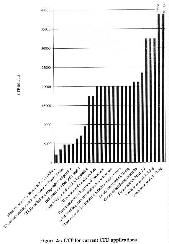
Table 20 provides a summary of specific CFD applications examined for this study:
110-114
| Machine | Year | CTP | Time | Problem | Problem size |
| IBM 360/67 | 1972 | 18 CPU hr | First 3D nonlinear transonic computation (STAGE II), over aircraft wing [40] |
100,000 grid points | |
| Cyber 203 | 1982 | 1-2 hours | SCRAMJET model [41 ] | 30 x 109 nodes | |
| Cray-1S | 1984 | 195 | 20 CPU hr | Simulation of after-body drag for a fuselage with propulsive jet. Reynolds averaged Navier-Stokes [40] |
|
| Cray-2 | 1984 | 1300 | 15 CPU m | Simulation of 2D viscous flow field about an airfoil [40] |
|
| Cray-2 | 1980s | 1300 | 100 CPU h | Simulation of external flow about an aircraft at cruise. Steady flow. Steady Navier- Stokes simulation. [42] |
1.0 million grid points. |
| Cray XMP/48 (1 Proc) |
1988 | 353 | 20-50 hr | Flow simulation around complete F-16A aircraft (wings, fuselage, inlet, vertical and horizontal tails, nozzle) at 6 deg angle of attack, Mach 0.9. Reynolds Average Navier Stokes. Reynolds number = 4.5 million. [43] |
1 million grid points, 8 Mwords (one 2 Mword zone in memory at a time), 2000-5000 iterations |
| Cray-2 | 1988 | 1300 | 20 hr | Simulation of flow about the space shuttle (Orbiter, External Tank, Solid Rocket Boosters), Mach 1.05, Reynolds Averaged Navier Stokes, Reynolds number = 4 million (3% model) [43] |
750,000 grid points, 6 Mwords. |
| Cray YMP/8 | 1989 | 3708 | Model of flow around a fully appended submarine. Steady state, non-viscous flow model. [39] |
250,000 grid points | |
| Cray YMP/1 | 1991 | 500 | 40 CPU h | Simulation of viscous flow about the Harrier Jet (operating in-ground effect modeled) [42] |
2.8 million points, 20 Mwords memory. |
| Cray C90/4 | 1993 | 5375 | 1 week | Modeling of flow around a smooth ellipsoid submarine. Turbulent flow, fixed angle of attack, [39] |
2.5 million grid points |
| CM-5/512 | 1995 | 20057 | 500 Timesteps |
Parafoil with flaps flow simulation. [44] | 2,363,887 equations solved at each timestep |
| CM-5/512 | 1995 | 20057 | 15,000 CPU sec, 30 CPU sec per each of 500 timesteps |
Flare maneuver of a large ram-air parachute. Reynolds number = 10 million. Algebraic turbulence model [44,45] |
469,493 nodes. 455,520 hexahedral elements. 3,666,432 equations solved per timestep. |
| CM-5/512 | 1995 | 20057 | Fighter aircraft (F-18?) at Mach 2.0. [44] | 3D mesh of 367,867 nodes, 2, 143,160 tetrahedral elements, and 1.7 million coupled nonlinear equations solved per timestep. |
|
| Cray T3D/512 |
1995 | 32398 | Modeling paratroopers dropping from aircraft. Moving grid. Cargo aircraft travelling at 130 Knots. High Reynolds number. Smagorinsky turbulence model [44] |
880,000 tetrahedral elements for half of the domain. |
|
| Cray T3D/512 |
1995 | 32398 | 500 timesteps | Steady-state parafoil simulation. 2 deg angle of attack. Reynolds number = 10 million. [44] |
38 million coupled nonlinear equations at every pseudo-timestep. |
| Cray T3D/512 |
1995 | 32398 | Fighter aircraft (F-18?) at Mach 2.0. [44] | 3D mesh of 185,483 nodes and 1,071,580 tetrahedral elements |
|
| Cray J916/1 | 1996 | 450 | 300 CPU hr | Modeling of transonic flow around AS28G wing/body/pylon/nacelle configuration. 3D Reynolds Averaged full Navier-Stokes solution. [46] |
3.5 million nodes, 195 Mwords memory |
| Cray YMP | 1996 | 500 | 8 CPU hr, 3000 timesteps |
Large-Eddy simulation at high Reynolds 3000 number [47] |
2.1 million grid points, 44 Mwords |
| Cray YMP/1 | 1996 | 500 | 6 CPU hr | Modeling of transonic flow around F5 wing (Aerospatiale). 3D Reynolds Averaged full Navier-Stokes solution. [46] |
442368 cells (192x48x48). |
| Cray C90/1 | 1996 | 1437 | 200 CPU hr | Simulation of unsteady flow about an F-18 High Alpha Research Vehicle at 30, 45, 60 deg angle of attack [48] |
2.5 million grid points for half-body modeling. 40 MWords memory |
| Cray C90/1 | 1996 | 1437 | 19 CPU hr | Simulation of turbulent flow around the F/A-18 aircraft at 60 degree angle of attack. Mach 0.3. Reynolds number = 8.88 million [49] |
1.25 million grid points. 100 Mwords of memory. |
| Cray C90/1 | 1996 | 1437 | 3 CPU hr | Modeling of flow over a blended wing/body aircraft at cruise. [50] |
45 Mwords of memory |
| Cray T3D/16 |
1996 | 2142 | 20,000 CPU sec. 50 CPU sec x 400 steps |
Aerodynamics of missile at Mach 3.5. Reynolds number = 6.4 million [51] |
500x150 (75,000) elements in mesh. 381,600 equations solved every timestep. |
| SGI PowerChallenge (R8000/150) /16 |
1996 | 9510 | 3.6 hr, 3000 timesteps |
Large-Eddy simulation at high Reynolds number [47] |
2.1 million grid points, 44 Mwords |
| Cray T3D/256 |
1996 | 17503 | 52,000 CPU sec. 130 CPU sec x 400 timesteps |
Aerodynamics of missile at Mach 2.5, 14- degrees angle of attack for laminar and turbulent viscous effects. [51] |
944,366 nodes and 918,000 elements. 4,610,378 coupled nonlinear equations solved every timestep. |
| Cray T3D/256 |
1996 | 17503 | 2 hr, 3000 timesteps |
Large-Eddy simulation at high Reynolds number [47] |
2.1 million grid points, 44 Mwords |
| CM-5/512 | 1996 | 20057 | 500 timesteps | Steady-state parafoil simulation, 10 deg angle of attack, Reynolds number = 10 million [37] |
2.3 million equations every timestep |
| CM-5/512 | 1996 | 20057 | 500 timesteps | Inflation simulation of large ram-air parachute, Box initially at 10 deg angle of attack and velocity at 112 ft/sec, 2 simulated seconds. [52] |
1,304,606 coupled nonlinear equations solved every timestep. |
| CM-5/512 | 1996 | 20057 | Flare simulation of large ram-air parachute. [52] |
3,666,432 coupled nonlinear equations solved every timestep. |
|
| CM-5/512 | 1996 | 20057 | 7500 CPU sec = 50 CPU sec x 150 timesteps |
Aerodynamics of missile at Mach 2.5, 14 deg angle of attack for laminar and turbulent viscous effects. [51] |
763,323 nodes and 729,600 elements. 3,610,964 coupled nonlinear equations solved in each of 150 pseudo-time steps. |
| Cray C916 | 1996 | 21125 | 3D simulation of flow past a tuna w/ oscillating caudal fin. Adaptive remeshing. Integrated with rigid body motion [33] |
||
| CM-5/512 | 1996 | 20057 | 3D simulation of round parachute, Reynolds number = 1 million [53] |
||
| IBM SP-2/ 32 |
1996 | 4745 | 80 minutes | 3D unsteady incompressible time-averaged Navier-Stokes. Multiblock transformed coordinates. [54] |
3.3 million points |
| CM-5/512 | 1996 | 20057 | 3D study of missile aerodynamics, Mach 3.5, 14 deg angle of attack, Reynolds number = 14.8 million [55] |
340,000 element mesh, nonlinear system of 1,750,000+ equations solved every timestep. |
|
| iPSC860/ 128 |
1997 | 3485 | 5 days | Small unmanned undersea vehicle. Fully turbulent model with Reynolds numbers. [39] |
2.5 million grid points |
| CM-5/512 | 1997 | 20057 | 30 hours | Parafoil simulation. [37] | 1 million equations solved 500 times per run |
| Cray C90/16 | 1997 | 21125 | 9 months | 3D simulation of submarine with unsteady separating flow, fixed angle of attack, fixed geometry [39] |
|
| Origin2000/ 64 |
1997 | 23488 | ARC3D: simple 3D transient Euler variant on a rectilinear grid. [29] |
||
| Cray T3E- 900/256 |
1997 | 91035 | 500 timesteps | Steady-state parafoil simulation, 10 deg angle of attack, Reynolds number = 10 million. [37] |
2.3 million equations every timestep |
| Origin2000/ 12 |
1997 | 4835 | 4329 sec | CFL3D applied to a wing-body configuration: time-dependent thin-layer Navier-Stokes equation in 3D, finite- volume, 3 multigrid levels. [30] |
3.5 million points |
| IBM SP-2/64 | 1997 | 7100 | 2 to 4 hours | Helicopter rotor free-wake model, high- order vortex element and wake relaxation. [23] |
|
| IBM SP-2/32 | 1997 | 4745 | Helicopter rotor motion coupled with rotor CFD, predict 3D tip-relief flow effect, parallel approximate factorization method. [23] |
||
| IBM SP-2/45 | 1997 | 6300 | 2 to 4 hours | Helicopter blade structural optimization code, gradient-based optimization technique to measure performance changes as each design variable is varied. [23] |
up to 90 design variables, one run per variable |
| Origin2000/192 | 1998 | 70368 | months | 3D simulation of submarine with unsteady flow, fixed angle of attack, and moving body appendages and complex repulsors. [39] |
Table 20: CFD applications
CFD Summary and Conclusions
The following conclusions can be drawn about CFD based on the preceding discussion:
Computational Chemistry and Materials
Computational chemistry, also known as molecular or particle dynamics, involves the study of the interactions of atoms and molecules. The interactions can span a wide range of forces. The particular field of study determines the forces studied in a computational run.
Particle Dynamics
In general, particle dynamic simulations mimic the motion of atoms. Individual atoms are represented in the simulation. These atoms may be bonded to other atoms to create molecules of varying size and complexity. The initial conditions for the simulation include the spatial coordinates of every atom, the bonds between the atoms making up the molecules, and the initial energies of the atoms (i.e., the atoms may already be in motion at the start of the simulation).
115
The simulation iteratively computes the total potential energy, forces, and coordinates for each atom in the system. These computations are repeated at each time step. The potential energy involves both bonded and non-bonded terms. Bonded energy terms derive from the energy contained within chemical bonds, and the motion of the atoms around the bond. Thus, the bonded energy terms consist of bond energy, angle energy, and dihedral-angle energy. The nonbonded energy terms derive from the forces that act between all atoms, whether bound together or not. These include van der Waals potentials (the attractive force between atoms or molecules of all substances) and the potentials that result from the electrical attraction and repulsion due to unbalanced electric charges.
Once the potential energy is computed for each atom, the forces acting on the atom are used to update its position and velocity. The new location and potential energy for each atom are stored and the process is then repeated for the next iteration.
The calculation of the non-bonded energy terms requires the largest percentage of the computational time. The non-bonded energy terms account for most of the calculation effort since the non-bonded energy of one atom is dependent on all the atoms in the simulation, both those nearby and those far away. This results in an n-squared problem where n is the number of particles in the simulation. By contrast, the bonded energy terms are relatively easy to compute, since each atom is bound to a small number of nearby atoms. In large organic molecules, the bonded energy terms become harder to compute. Protein folding, for example, models molecules that have at least 10,000 atoms. Since the protein can fold in a number of ways, it becomes nontrivial to determine which atoms are "nearby".
The algorithmic efforts in particle simulations have primarily been directed at the non-bonded energy terms. As the number of particles in the simulation grows, the effort to compute the nonbonded energy at each step potentially grows as n2. Simulations involving hundreds of millions of atoms are not uncommon. In fact, such simulations still represent relatively small amounts of atoms, relative to Avogadro's number (6.023 x 10²³)18. The usual technique employed to reduce the computation time is to ignore the contribution of atoms far away. Atoms beyond a certain distance are either not included in the computation, or are included only as an aggregate value representing all distant atoms in a given direction.
The number of particles desired in simulations and the computational requirements combine to make parallel machines the primary choice for particle simulations. The straightforward approach to the simulations is to divide the simulation space evenly across the processors, with each processor performing the calculations for particles that are within its space. For simple simulations, this usually suffices. Each processor will communicate with other processors on each time step to get updated information about the other atoms. For simulations that ignore the far-field effects of atoms, each processor need only communicate with those processors nearest in the simulation space. These communications have to convey the locations of all the atoms for
____________________
18 Avogadro's number is the number of particles (6.023 x 10²³) present in an amount of a compound that is equal to the atomic weight. For example, 12 grams of carbon (just under one-half ounce) would have 6.023 x 10²³ carbon atoms.
116
each processor, since each of these atoms need to be considered in computing the updated energies for the atoms the processor is responsible for.
When far-field effects are included, the communication increases. However, it does so gradually. Only aggregate position and energy values need to be communicated by each processor to the distant processors. In some simulations, the processors are grouped into regions and only the data for the region is sent to the distant processors.
This simple view is inadequate when the particles in a simulation may be subject to widely varying densities across the simulation space, for example, a simulation where particles are attracted to electrodes. A simulation that starts with an even distribution of particles across the region, and a balanced workload for the processors, will gradually find more particles being handled by the processors that are near the electrodes, while other processors away from the electrodes are left idle. Such load imbalances can be corrected by varying the region for which each processor is responsible. Changing the region size and re-distributing the particles takes time. Thus, the frequency of the load balancing has to be matched in some way with the motion of the particles. When the load balancing is not done often enough, processors are idle too much of the time. When the load balancing is done too often, the load balancing itself begins to use too much of the computation time.
Explosions
In addition to considering the classical dynamics interactions of particles colliding (as described above), explosions must consider the chemical changes in the molecules themselves. These changes release energy into the system that results in a reaction wave that travels through the explosive material at hypersonic speeds, ranging from 1-10 km/sec. Molecular simulations of the shock wave propagation have been done since the 1960's. Studies of shock-initiated systems have been done since the 1970's. However, these were very simple models, and not able to do justice to the complex chemical processes present when using modern explosives.
The Department of Defense is a major source of research funds for explosive simulations. The Army, for example, is studying solid chemical propellants used to fire projectiles. The objective is to propel the shell from the gun but with minimal damage to the barrel. Some work is being done, on non-solids, for example, the use of liquid propellants that are inert until mixed in the barrel. The Federal Aviation Administration provides some support in the area of fuel-air explosive mixtures for the purpose of designing better fuel systems for aircraft.
An ability to simulate explosions at the molecular and atomic level can provide the following benefits:
117
An explosive simulation solves two basic sets of equations The first set is the classical equations of motion for the N atoms present in the system. These equations will provide the kinetic energy for the system. The second set is the potential energy within the molecule in the form of the internuclear distances and bond angles. This potential energy becomes the most computationally intensive part of the simulation.
The simulation describes a reactive medium through which the reactive wave will pass. The medium is often described as a perfect, or near perfect, set of small crystals of diatomic atoms. This model is deliberately too simple, as the techniques for handling realistic explosive molecules are not yet in place. Thus, a two-atom molecule is used in the explosive, rather than the large and complex organic molecules that make up current explosives. In addition, it is believed that hot spots within the material play an important role in detonation. Such hot spots can result from shear stress and defects in the crystal, for example. Some simulations have attempted to incorporate such effects. However, explosive simulations remain quite simple.
To achieve better simulations, several issues must be addressed. First, explosives are large organic molecules that undergo several changes during an explosive. Each change involves creation of intermediate compounds, which react to continue the explosive release of energy. Second, imperfections in the crystalline structure are believed to contribute significantly to the explosion, but are seldom modeled. Finally, differences in compression of the crystal and initiation of the shock wave have not been well represented in current models [56].
Within the past five years, two-dimensional models have been developed. These models use diatomic molecules, and have up to 10,000 molecules in a simulation. The model will initiate a shock wave at one end of the two-dimensional grid of molecules, then follow the shock wave through the material. One of the difficulties is having a long enough crystal in the direction of the shock wave. The crystal will undergo several distinct phases as the shock wave approaches and passes each section. First, the molecules are disturbed from the initial positions. Then they undergo disassociation. Simulations have suggested that the molecules form intermediate polyatomic products that then decompose releasing heat. Finally, the end products of the reaction are formed as the tail of the shock wave passes. The small simulations run to this point are already showing unexpected results in the vicinity of the shock wave. The polyatomic intermediate products, for example, have appeared in simulations, but have not been observed in actual live explosions. Additional work is underway in the area of quantum mechanics. The classical mechanics effects are well developed in the models, but the quantum effects still need work.
Current simulations are running on platforms that generally are below the current export thresholds. Some examples include [57]:
1992 IBM RS6000 model 550, single processor, one month run (less than 500 Mtops)
1997 SGI PowerChallenge, 4 processor, overnight run (1686 Mtops)
The PowerChallenge code is moderately scalable to 4 processors. It continues to see shorter run times to 16 processors; however, the growth curve is decidedly sub-linear. Above 16 processors, the code exhibits negative growth. In part, this is a load balancing issue, since a large amount of
118
work is located within the shock wave and the shock wave is moving rapidly through the crystal It is difficult to concentrate sufficient processor power on the area of the shock wave without encountering excessive communication costs.
Such simulations are only a first approximation. Realistic models need a minimum of 20 to 30 atoms per molecule and at least 30 to 40 thousand such molecules in a three-dimensional model.
The performance listed above is for a two dimensional code that includes only the classical dynamics. An area of intense research is how to fit the quantum mechanics into the simulations. In an explosion, there are too many variables to be able to solve the equations adequately. Quantum mechanical reactions in solids have not been done; researchers are currently working from first principles. Researchers at the Army Research Laboratory, Aberdeen, are using Gaussian94 [58]. It is designed to handle the quantum mechanical effects--molecular structures, vibrational frequencies, etc.--for molecules in the gas phase and in solution. ARL is adopting the code for use with solid explosives.
A primary computational consideration for these simulations is storage space, both in main memory and secondary storage. The space requirement scales with the number of atoms for the classical dynamics. For the quantum mechanics, the space requirement scales as the number of electrons to the fifth power (n5). The quantum mechanics integrals are used repeatedly during a simulation. The common technique is to compute them once, then store the solutions for use during the simulation. These temporary files can occupy 30 to 40 gigabytes of disk space on workstation implementations. Historically, the disk space requirement has driven the use of vector machines for these simulations. Now, desktop and small parallel systems can be used if equipped with sufficient disk space.
A secondary problem with scaling to larger problems is a visualization problem. There are not any codes suitable for viewing a three-dimensional explosion. Most visualization tools today are oriented toward volumetric data rather than particle data. The primary technique for viewing large numbers of particles is to reduce the data set by eliminating some fraction of the particles, or combining them into representative particles. With an explosion, this is not sufficient, since the researcher is particularly interested in what is happening in the area of the highest concentration, and greatest volatility; i.e., the shock wave.
Performance measurements
Table 21 shows the performance of a variety of computational chemistry problems over time.
119-120
| Machine | Year | CTP | Time | Problem | Problem size |
| CrayXMP/l | 1990 | 353 | 1000 hours | Molecular dynamics of bead-spring model of a polymer chain [59] |
Chainlength = 400 |
| Cray YMP | 1991 | 500 | 1000 hours | Modeling of thermodynamics of polymer mixtures |
lattice size - 1123
chain size = 256 |
| Cray YMP | 1991 | 500 | 1000 hours | Molecular dynamics modeling of hydrodynamic interactions in "semi- dilute" and concentrated polymer solutions |
single chain
60 monomers |
| Cray C90/2 | 1993 | 2750 | 12269 sec | Determination of structure of E. coli trp repressor molecular system [60] |
1504 atoms
6014 constraints |
| CM-5/512 | 20057 | 8106 sec | |||
| Cray C90/2 | 2750 | 117 sec | 530atoms
1689 distance & 87 |
||
| CM-5/256 | 10457 | 492 sec | |||
| Cray C90/1 | 1993 | 1437 | .592 sec/ timestep |
MD simulation using short-range forces model applied to 3D configuration of liquid near solid state point [61] |
100,000 atoms |
| Intel iPSC860 64 nodes |
2096 | 3.68 sec/ timestep |
1 million atoms | ||
| Cray T3D/256 | 17503 | 1.86 sec/ timestep |
5 million atoms | ||
| Intel Paragon/1024 |
24520 | .914 sec/ timestep |
5 million atoms | ||
| Intel Paragon/1024 |
24520 | .961 sec/ timestep |
10 million atoms | ||
| Intel Paragon/1024 |
24520 | 8.54 sec/ timestep |
50 million atoms | ||
| Cray T3D/512 | 32398 | .994 sec/ timestep |
5 million atoms | ||
| Cray T3D/512 | 32398 | 1.85 sec/ timestep |
10 million atoms | ||
| IBM SP1/64 | 1993 | 4074 | 1.11 sec/ timestep |
Molecular dynamics of SiO2 system [62] | 0.53 million atoms |
| Intel Touchstone Delta/512 |
13236 | 4.84 sec/ timestep |
4.2 million atoms | ||
| Paragon 256 | 1995 | 7315 | 82 sec/ timestep |
Particle simulation interacting through the standard pair-wise 6-12 Lennard- Jones potential [63] |
50 million particles |
| Paragon 512 | 1995 | 13004 | 82 sec/ timestep |
100 million particles | |
| Paragon 1024 | 24520 | 82 sec/ timestep |
200 million particles | ||
| Paragon 1024 | 24520 | 82 sec/ timestep |
400 million particles | ||
| SGI PowerChallenge 4 nodes |
1997 | 1686 | overnight | Explosion simulation [56] | 30 thousand diatomic molecules |
Table 21: Computational chemistry applications
The length of a run is generally dependent on two factors: the time the researcher has available on the platform and his patience. Disk storage space available is a third, less significant factor. The more disk space available, the more often the simulation can save the current state for later visualization
Conclusions
The discussion of computational chemistry leads to the following conclusions:
121
Computational Structures and Mechanics
Since the military use of gunpowder started in Western Europe, there has been an on-going race between the development of structures that are able to withstand high velocity projectiles and improved projectiles designed to penetrate such structures. The advent of armored ships during the last century and the development of armored vehicles in this century have extended this race to include structures on the move. As a result, the military has long been keenly interested in the study of structural mechanics. In the past, this study has been carried out through extensive costly and dangerous field-experiments. These experiments are still necessary today, however, the growing power of high performance computers has given rise to the use of Computational Structural Mechanics (CSM) to both supplement and extend the results of field experiments.
Two specific application areas that arise from this work were studied for this project: the response of earth and structures to the effects of explosive loading and the impact of projectiles in earth, structures, and armor (also known as armor/anti-armor). For both projects, a judicious combination of experiments and computer simulations is used to characterize the dominant physical phenomena. In addition, the computer simulations provide insight into transformations occurring during the experiments that cannot be observed due to the extreme conditions. Finally, computer simulations help direct subsequent rounds of field experiments.
Survivability of structures
Structure survivability involves research in four areas:
This work investigates the offensive use of weapons to penetrate, damage, and destroy buildings. It also looks at the defensive features of buildings that make them more resistant to the effects of various types of weapons.
During the Cold War, much of the effort in this field was devoted to studying the effects of nuclear blasts and how to design structures to withstand such explosions. Since the end of the Cold War, and in particular since the Gulf War, the work has focused more on the effects of conventional munitions and the ability of structures to withstand such explosions.
Two types of weapons effects are studied. The first is the effect of conventional explosions on various types of structures. The second is the study of the ability of various types of projectiles to penetrate through layers of natural and man-made materials.
Conventional Explosions
A conventional explosion is a highly non-linear reaction. To model it in three dimensions, a finite volume (FV) technique is used with a structured grid. The technique is to follow the strong
122
shock wave interference as it moves outward from the source of the explosion through a grid of cells that fill the space. The pressure can be determined from the shock wave front at any point as the wave moves outward. At points where the shock wave encounters the ground or a structure, the pressure can be used to determine how the ground or building will respond to the blast. The response, of course, is limited by complexity of the numerical model used to represent the material.
To accurately calculate the pressure, a very fine mesh is needed in the vicinity of the shock wave. However, it is not feasible to use such a fine mesh throughout the problem space due to both the computational and memory requirements that would be imposed. Therefore, as the shock wave moves outward, the grid needs to be re-meshed to keep a sufficiently fine mesh near the shock front. The current state-of-the-art is to re-mesh after a pre-determined number of time steps. Adaptive meshing techniques, that automatically re-adjust the mesh when needed, are a current area of study.
The time integration step for studying explosions or high-strain rate material behavior is very small. Typically, stability criteria limit time steps to the sub-microsecond regime. The total time simulated is based on the duration of the explosion or impact event. Many conventional air blast simulations are run for tens of milliseconds, while high-velocity projectile impacts are on the order of several hundred microseconds. There is a direct relationship between the time scale and the resolution (i.e., the size of the cells used in the finite volume technique). Since the computation is following the shock wave through the cell, a time step is needed such that the wave does not travel through more than one cell. Thus, doubling the resolution will raise the computational workload by a factor of 16. Doubling the resolution in each of the three dimensions adds a factor of 2, for a total of 8. Halving the size of the time step adds another factor of 2.
CTH is one code used for modeling the expansion of the shock wave outward from an explosive device. CTH is an Eulerian hydrodynamic code, uses a structured mesh, and computes shear stresses. It provides the pressure due to the shock wave in any of the cells during the simulation. This pressure can then be used to determine the effect of the blast on the ground and building(s) in the vicinity of the explosion. CTH is used in nuclear and armor/anti-armor applications (see below for both) as well as structural problems.
Originally developed for use on parallel vector processors, CTH took advantage of microtasking to utilize the available processors. It has been ported to parallel machines and now runs on everything from a single-CPU PC to the largest parallel machines (i.e., Origin2000, T3E, and ASCI Red). It uses a strictly data parallel programming model. The main difficulty in the parallel port was determining the domain decomposition strategy. Each processor is assigned a subdomain (50 x 50 x 50 is typical). A set of ghost cells surrounds the sub-domain. The processor executes within its sub-domain as though it were the only processor. Message passing is used to exchange data from the ghost cells between adjacent sub-domains. [64].
123
Structural Response
Modeling the effect of an explosion on a building imposes two fundamental problems. The first is a time scale problem. The explosive shock wave requires microsecond time scales. The building response however. is on a second to minutes time scale. Thus, it may take 10 to 100 microseconds for the shock wave to reach and surround a building, several seconds for the structure of the building to begin to respond to the shock wave, and up to a minute for the building to collapse. The one exception to the time scale difference is the response of glass to a shock wave. If the shock wave is sufficient to shatter the glass, this will happen on the same microsecond time scale the shock wave simulation is using.
The second fundamental problem is the different techniques used to model structural response and shock wave propagation. Structural response uses a non-linear Lagrangian code operating on a finite element (FE) mesh. DYNA3D is a code used extensively in a variety of structural applications. For use in survivability calculations, the code has incorporated numerical models which better reflect the use of brittle materials such as concrete and mortar that are often present in military and other hardened structures.
Ideally, the conventional explosion and the structure simulations should be coupled. This would allow a more accurate and realistic determination of the effect of a blast on a structure. Work is proceeding on coupling the CTH and DYNA codes. An approach being used is to develop a combined solver, the Arbitrary Lagrangian Euler (ALE) formulation currently under development by DoE as part of the ASCI project. Estimates are that it will take four to five years to get the coupling accomplished. This time frame is due in part to the difficulty imposed by the different solution techniques. It is also due to the realization that no current machine would be capable of performing the calculation. It is expected that advances in computing technology will provide such a machine within five years.
Performance points
Water over C4 explosive in container set above wet sand [65]:
Alternate scenario: longer simulated time, fewer cells [65]
Explosion engulfing a set of buildings [66]:
124
Hardened structure with internal explosion [67]:
Impact of projectiles on armor
Armor/anti-armor simulations study the effectiveness of armor protection for vehicles and buildings and the lethality of projectiles designed to penetrate such armor. Traditionally, this work has been based on actual field experiments. Over the past two decades, computer simulations have become increasingly useful in these studies. Initially, the simulations attempted to replicate the results of field experiments. These early simulations were two-dimensional and could model only simple impacts, such as a projectile hitting the armor at a right angle. As improved machines became available, these simulations have been expanded into three dimensions and are now able to model impacts at a variety of angles. The simulations also model more realistic armor, including multi-layer armor, and simulate targets that reflect the curvature and slope of actual armor. Today, the simulations are helping to shape the field experiments that are conducted and allowing researchers to make more effective use of the field experiments.
Penetration mechanics
The impact of a high-velocity projectile on an armor target generates a hypersonic shock wave that moves outward from the point of impact through the material of the armor. The shock wave
125
will deform both the armor and the projectile. Approximate analytical methods are available for studying this problem, but suffer from the simplifying assumptions they must make. If a computational approach is to yield a satisfactory and complete description of the impact and its effects, a numerical solution is essential. The numerical approach uses finite difference and finite element methods in finding solutions to the partial differential equations. If a complete description is desired, the solution must account for the geometry of the projectile and target, the materials of which each is composed, and the propagation of the hypersonic shock wave that moves outward from the point of impact. This hypersonic shock wave is very similar to the shock wave in air that was explained above in the description of the structure survivability work. The shock wave causes dramatic changes in the material comprising the armor, including changes of state that require the inclusion of hydrodynamic forces. Finally, the projectile and target will deform under the impact, and the initiation and propagation of this deformation must be included in the numerical approach [68].
Computational constraints
Solutions to such penetration mechanics problems are both computation and memory intensive. A fine scale mesh is needed to accurately represent the hypersonic shock wave moving outward through the armor target and the projectile. Increasing the resolution of this mesh improves the accuracy of the simulation. However, the same problem is encountered here as in the explosive study described above. To double the resolution requires a 16-fold increase in computational cycles, and an 8-fold increase in the number of cells in the mesh. Doubling the resolution requires twice as many cells in each of the three dimensions, thus the 8-fold increase in memory size. The time step must be halved when doubling the resolution. This requirement comes from the restriction that the shock wave should not move further in one time step than the size of one cell. Halving the size of the cell thus requires a halving of the time step.
A variety of effects need to be included in the computation:
All of these contribute to the time needed to perform the calculations on each time step.
The early (1970's) simulations in this field modeled two-dimensional impacts. The projectile struck the target at right angles to the surface, and the target was represented as a flat plate. Neither of these restrictions is realistic in combat. Armor faces are both curved and sloped in an effort to deflect the projectile and diminish its effectiveness. If a simulation is to be realistic, it must take into account the actual shapes used for armor and the likelihood that the shell will impact at an angle other than 90 degrees.
The transition from 2-D to 3-D greatly increases the memory requirements and the time needed to find a solution. 2-D simulations require a few tens of thousands of cells. The early 3-D
126
simulations started at half a million cells. Today, simulations using tens of millions of cells are common. with demonstration projects using up to one billion cells. Simulations in the tens of million-cell range can require l00 to 400 hours of computer time.
Parametric studies
Much of the real benefit in running these simulations comes from parametric studies. Such studies use multiple runs varying the parameters of interest. For example, a series of runs might vary the angle of impact, the velocity of the projectile, and/or the composition of the target or projectile. It is the need for parametric studies that results in the gap between demonstration projects that are run once as a proof-of-concept, and the size of the more common projects where multiple runs can be made.
Performance points and history
In the 1970's, the Cyber machines supported 2-D simulations involving tens of thousands of cells. These simulations had simple projectile and target geometries and included some elastic constituative models. The limiting factor in the transition to 3-D simulations was insufficient memory.
The 256 Mword memory of the Cray-2 provided sufficient memory to begin doing 3-D simulations involving 0.5 to 1.5 million cells. At first, the simulations were run using only one processor, with the other three idle to allow access to the entire memory of the machine. Later, the code (CTH) was modified to take advantage of Cray's micro tasking to allow all four processors to work on the simulation.
Today, a transition is in progress to MPP platforms. The transition has been slow due to the uncertainty as to which platform, and which programming tools, would be successful. The development of PVM and MPI, and their support by the various vendors, has spurred the changeover to a massively parallel platform. Deciding how to handle the domain decomposition of the problem was the biggest task in the PVP to MPP move. The CTH code is the primary code used in this work; this is the same CTH code used in the structure survivability work described above. The code now runs on a variety of platforms, from workstations to PVP to MPP. The workstation versions of the code are sufficient for 2-D computations--an example of an application that used to require the highest level of computing, but now runs on much smaller platforms.
Future work
127
Computational geomechanics
Computational geomechanics simulates soil-structure interactions. Example simulations include vehicle-ground interaction, pile driving, and mass movements by avalanche. In the context of national security issues, an example application is the "Grizzly", a special purpose M- I tank chassis that will serve as a breaching tool to clear paths through mine fields, wire, rubble, and other obstacles A plow attached to the Grizzly is being designed to clear a path by lifting antipersonnel mines and pushing them to either side. Computer simulation potentially allows the testing of the plow in a variety of soil and terrain conditions, and against a variety of mine types. Potential benefits of the simulations include improvements in the design of the plow and testing of the plow in various conditions without the need and cost to transport the prototype tank to different locations.
Soil-structure interactions can result in the soil behaving as though in different "phases". These phases mirror the solid-liquid-gas phases that matter typically occupies. For the "solid" phase, the soil behaves as a large solid, or a small number of large solids. For the "liquid" phase, such as occurs in an avalanche or a mudslide, the soil behaves very much like a liquid flowing in a current. For the "gas" phase, the soil behaves as individual particles moving independently. No one model is currently able to handle these different phases [69].
The mine plow application models the soil as independent particles that interact with each other when they come into contact; a technique know as a Discrete Element Model (DEM). The technique has similarities with that described earlier for molecular dynamics. It is based on the application of Newton's Laws of Motion to the individual particles. Unlike molecular dynamics, only those particles in actual contact with the particle of interest can affect its motion. The particles used in these simulations are much larger than the atoms and molecules used in molecular dynamics. Particles here can be as small as individual grains of sand or other soil particles and range upwards in size to represent rocks, mines, etc.
The acceleration of each particle for a specific time step is found by first computing the total force on the particle. Once the force is known, Newton's laws of motion are integrated across the time step to determine the current velocity of the particle. The total force acting on a particle is the combination of two types of forces. The first type is in the direction of the particle's motion and due to physical contact with other particles. This force is treated very much like a spring, either compressing as the two particles move closer together, or releasing as the particles separate. The second type of force occurs in directions perpendicular to the motion of the particle. This force is also modeled as a spring, but with the addition of a frictional slider.
For the plow simulation, the overall computation uses three steps:
1) calculating the force applied by the plow blade and boundary conditions,2) calculating the interaction forces between particles, and
128
3) integrating to obtain the revised motion of the particles
One of the largest computational burdens is imposed by the need to determine which particles are in contact with each other. The simplistic approach of looking at all possible particle-particle pairs leads to an untenable n-squared problem A better, linear solution uses a cell method of dividing the particles in a 3-dimensional grid of cells. Particles that touch a particular particle can then be located only in the particle's own cell, or in cells that immediately adjoin the particle's cell A neighbor's list is updated for each particle, and the cell size is set large enough to handle the largest particle present in the simulation.
Domain decomposition on parallel platforms is done in the two horizontal directions, creating a set of columns, each of which is assigned to a processor. Care has to be taken when assigning particles to cells as the simulation progresses to avoid having a small numerical error result in the particle seeming to be in two cells at once. Having the owning cell determine ownership for the new position of the particle solves this.
Current runs are examining tens of thousands of particles, typically 40K to 100K. The need is for runs that can handle several million particles and to perform a parametric study. The work over the next year will examine different soil conditions, mine types, and other obstacles within and on top of the soil. It will also allow study of the effect of varying terrain.
In addition to the computational resources, researchers are looking for solutions to the analysis of the simulations. Visualization techniques do not adequately support particle counts in the million plus range. Reduction algorithms are needed to lower the number of particles actually rendered. These reduction algorithms can be time consuming in their own right. Attempts to do near realtime simulations with small numbers of particles have required almost as much computing power for the reduction algorithms as for the particle dynamics. In off-line analysis, smaller computers can be used for the data reduction, but will add considerably to the total time required to produce the visualization.
Performance points
Table 22 shows performance points for a number of structural mechanics problems. Historical data is included to show the progression of problem sizes and computational requirements over time.
129-130
| Machine | Year | CTP | Time | Problem | Problem size |
| Cyber | 1980 | 2D modeling of simple projectile striking simple target. [70] |
10,000s of grid points | ||
| Cray-2/l | 1987 | 1300 | 400 hours | 3D modeling of projectile striking target. Hundreds of microsecond timescales. [70] |
.5-1.5 million grid points 256 Mword memory |
| Cray YMP/1 | 1990 | 500 | 39 CPU sec | Static analysis of aerodynamic loading on solid rocket booster [71] |
10,453 elements, 9206 nodes, 54,870 DOF19 256 Mword memory |
| Cray YMP/2 | 958 | 19.79 CPU sec | |||
| Cray YMP/4 | 1875 | 10 CPU sec | |||
| Cray-2 | 1992 | 1300 | 5 CPU hours | Modeling aeroelastic response of a detailed wing-body configuration using a potential flow theory [71] |
|
| Cray-2 | 1992 | 1300 | 6 CPU days | Establish transonic flutter boundary for a given set of aeroelastic parameters [71] |
|
| Cray-2 | 1992 | 1300 | 600 CPU days | Full Navier-Stokes equations [71] | |
| C916 | 1995 | 21125 | 900 CPU hours | Hardened structure with internal explosion, portion of the overall structure and surrounding soil. DYNA3D, nonlinear, explicitly, FE code. Nonlinear constituative models to simulate concrete & steel. [67] |
144,257 solid & 168,438 trust elements for concrete & steel bars, 17,858 loaded surfaces, 500,000 DOF, 60 msec simulated time |
| Cray C912 | 1996 | 15875 | 435 CPU hours | Water over C4 explosive in container above wet sand, building at a distance[65] |
13 million cells, 12.5 simulated time |
| Cray C912 | 1996 | 15875 | 23 CPU hours | Water over C4 explosive in container above wet sand, alternate scenario: container next to building, finite element [65] |
38,000 elements, 230 msec simulated time, 16 Mwords memory |
| Cray C916 | 1996 | 21125 | 325 CPU hours 3 day continuous run |
Explosion engulfing a set of buildings, DYNA3D analysis to study effects on window glass & doors done off-line after the blast simulation completed [66] |
825 Mwords memory |
| workstation | 1997 | 500 | 2D model of simple projectile striking simple target. [70] |
10,000s of grid points | |
| Cray T3E-900 256 nodes |
1998 | 91035 | 450,000 node hours |
Grizzly breaching vehicle plow simulation, parametric studies, different soil conditions & blade speeds [72] |
2 to 4 million particles (soil, rock, mines, obstacles, etc.) |
Table 22: Structural mechanics applications
Conclusions
The preceding discussion leads to the following conclusions:
Computational Electromagnetics and Acoustics
Introduction
Computational Electromagnetics and Acoustics is the study of the electromagnetic (light) and acoustic (sound) properties of physical objects by computationally finding multi-dimensional solutions to the governing electromagnetic or acoustic equations. Such studies find applications in the design of tactical vehicles and antenna design, the development of laser systems, the detection of buried munitions such as mines, and other areas. A great deal of the attention in this area is focused on determining how "visible" an object such as an aircraft or a submarine is to various forms of electromagnetic or acoustic sensing devices, such as radar or sonar. Such studies focus on the nature of electromagnetic or acoustic energy generated from an outside source and reflected by the object in question. Other studies focus on the nature of the emitted energy of an object. For example, the acoustic signature of a submarine is a description of the way the vibration caused by the subs mechanical parts interacts with the sub's construction and the surrounding water to produce acoustic waves that can be picked up by remote sensors. This section focuses on two applications in particular, radar cross sections and acoustic signatures
131
Radar Cross Section
Overview of Radar Cross Section
The radar cross section is the measure of a target's ability to reflect radar signals in the direction of the radar receiver where they can be sensed The magnitude of a target's radar cross section, and hence its visibility to the radar system, is a function of the target's projected profile, its reflectivity, and its directivity. The projected profile can be thought of intuitively as the size of the shadow of the target in the presence of a light source emanating from the radar source The reflectivity is the percentage of the radar's power reflected back in the direction of the radar receiver. The directivity is the ratio of the power reflected back toward the radar receiver to that which would have been reflected back by an object (like a sphere) that reflects uniformly in all directions. Figure 26 shows the reflection from various shapes.
Reducing a target's radar cross section has a direct impact on its survivability. A reduced radar cross section not only makes the target more difficult to detect, it reduces the amount of power needed to generate jamming signals to counter the radar signals. Efforts to reduce a target's radar cross section focus on altering the external shape, utilizing special absorbent materials, or taking measures to alter the nature of the reflected signal. Some external design changes seek to minimize the projection profile, especially in the directions from which radar signals are most likely to come (e.g. from the front, or from below). Other design changes seek to reduce the directivity by using tilted or rounded surfaces that reflect less energy back to the radar source. Using materials or colors that better absorb the electromagnetic waves at the frequencies more likely to be employed by radar can reduce reflectivity. For example, a surface painted black reflects much less visible light than does that same surface painted white. More sophisticated materials and techniques are needed for the frequencies typically used in radar systems. Generating jamming signals whose electromagnetic characteristics nullify those of the reflected signal can also reduce radar reflectivity.
132
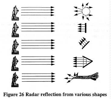
If the radar signal wavelength is much smaller than the radius, a perfect sphere's radar cross section is independent of the wavelength and frequency of the radar signal, and is computed as the area of the cross section of the sphere (pir2 ). Other shapes may have different radar cross sections depending on the frequency of the radar signal. For example, a flat plat has a radar cross section equal to 4pia2/lamda2, where a is area of the plate, and lamda is the wavelength, which is inversely proportional to the frequency. Therefore, a given plate will have a radar cross section that is one hundred times (102) larger under a 10 GHz radar signal, than under a 1 GHz signal, since a 10 GHz signal has a wavelength one tenth as long as a 1 GHz signal.
The reflective nature of simple geometric shapes is well understood, and the corresponding radar cross sections can be solved using analytic means. Targets such as ships and aircraft are geometrically very complex, however. They have a great many reflecting surfaces and corners of varying shapes. Not only are their shapes too complex to solve analytically, but only within the last year has it become possible to compute the radar cross section for an entire aircraft for any frequency approaching that used in operational systems [73]. In practice, the radar cross section is measured after a scale model of the vehicle has been built. Necessarily, these tests are made rather late in the design process. Modifications to the target's shape at this point are usually costly to implement. The ability to compute radar cross sections for realistic shapes is very desirable in large part because it would make it possible to evaluate accurately the results of a candidate design early in the design process, when changes are inexpensive and easy to make.
Computational Nature of Radar Cross Sections
Calculating the radar cross section computationally involves solving numerically from first principles the partial differential or integral Maxwell equations. These equations describe the properties over time of changing electric and magnetic fields (light, radio. radar) through media with various refractive and permeability properties.
133
One leading approach to solving these equations is called a characteristic-based method As in many computations from the field of computational fluid dynamics, characteristic-based electromagnetics computations define a system with a set of initial values. and compute the state of the system over space and time, one time-step at a time The evolution of the system can be thought of as tracking the movement of information representing changing electric and magnetic fields in time and space. These trajectories are called characteristics [74]. To set up a characteristics-based solution method, the three-dimensional domain being modeled it represented by a set of grid points (for a finite difference method) or cells (for a finite volume method). Each grid point/cell consists of the variables dictated by the governing equations and, depending on the algorithm, additional memory locations for storing the flux, or rate of change of the fields. There are six dependent variables and three spatial independent variables with nine directional variables. Adding in the memory locations for the flux values, nearly 50 memory locations per grid point/cell are required.
The computational demands of such problems can be enormous. To obtain the necessary numerical resolution, cells must be no larger than one-tenth the wavelength of the radar. This requires at least ten elementary finite volume cells (or ten nodes in a finite difference approach) for each wavelength. The greater the frequency of the radar signal, the smaller the wavelength, and the finer the mesh must be. In high frequency radar beyond the X Band (approximately 10 GHz), the wavelength is reduced to a centimeter or less. Modeling an aircraft with a wingspan of 10 meters requires 10 meters x 100 centimeters/meter x 10 cells/centimeter = 10,000 cells in each dimension, or 10,0003 = 1 trillion cells. Since each cell consists of approximately 50 variables, for this kind of simulation, approximately 50 trillion variables are manipulated. In each time-step, hundreds of trillions of operations are needed to advance the computation a single timestep. If multiple viewing angles or multiple frequencies are to be computed, the computational requirements are astronomical [75].
A "holy grail" of computational electromagnetics has been the computation of the radar cross section of an entire modem fighter aircraft for a fixed incident angle and a 1 GHz radar signal. While this frequency is less than the 3-18 GHz of normal radar, it is nevertheless an important milestone. Only recently has a problem of this size come within the reach of available computing platforms. At 10 cells points per wavelength, 50 million are needed for a modeling space of 15 meters x 10 meters x 8 meters. On a single-processor Cray Y-MP advancing the computation a single time-step would require nearly four hours of compute time. -Completing a single simulation requires 500 or more timesteps and multiple viewing angles, or months of compute time [76].
Since the mid-1990s, availability of scalable multiprocessors with high-bandwidth, low latency interconnects has opened up avenues of substantial progress in the field [74]. While the large number of available CPU cycles is certainly a benefit on massively parallel systems, the large memory space is even more beneficial [77].
A central task in running the application on a parallel system is determining how to partition the domain to balance the load across processors, and minimize the amount of inter-node communication needed. The subject of the best way to do this is a matter of on-going research.
134
One simple. but not necessarily optimal, approach that has been used productively is to partition the three dimensional domain into a set of planes as shown in Figure 27 [75,76].

Each plane is assigned to a processor. In each timestep, grid points/cells exchange values with their neighboring grid points/cells. The amount of data exchanged between nodes is therefore directly proportional to the number of grid points/cells in each node. In addition, each computing node must issue a minimum of two global synchronization operations. In short, although the problem partitions nicely, a considerable amount of communication does take place, and some studies have indicated that the capability of the interconnect is the factor most limiting scalability. Up to the point where the interconnect becomes saturated this kind of problem exhibits well over 90% scaling, if the problem size is increased as the number of processors grows. The point at which saturation occurs varies from model to model, but in the range of 128256 nodes for the Cray T3D, Intel Paragon, and IBM SP-2. [75,78,79].
Are tightly coupled multiprocessors absolutely necessary for solving computational electromagnetics problems? Strictly speaking, the answer is no, for many applications. However, the better the interconnect, the better the obtainable performance. Loosely coupled systems can solve problems. Timely solutions require homogeneous, tightly-coupled systems [77]. Moreover, the difference between military and civilian computational electromagnetics computation is not so much fundamental differences in the applications or numerical methods employed, but rather in the extreme nature of military usage. While designers of a civilian aircraft may be interested in the radar cross section for a specific radar frequency employed by flight controllers, designers of a military aircraft would be more interested in the radar cross section across a host of possible radar frequencies. The additional demands of military applications create a need for the more tightly coupled high performance systems.
The field of computational electromagnetics continues to evolve rapidly. New numerical methods, domain partitions, and computational platforms have made previously unsolvable problems accessible. For example, researchers at the University of Illinois at Urbana/Champaign have used an Origin2000 to compute the radar cross section of the VFY218 aircraft under a radar
135
wave of 2 GHz, becoming the first to do so at this frequency [80]. The equations solved contained 1.9 million unknowns. The breakthrough was the development of very efficient algorithms for calculating the scattering of radar waves off large objects.
| Machine | Year | CTP | Time | Problem | Problem size |
| Cray YMP/1 | 500 | 5 CPU hr per timestep |
Signature of modern fighter at per fixed incident angle at 1GHz [76] |
50 million grid points @ 18 words/grid point |
|
| Cray C916 | 1994 | 1437 | Radar cross section on perfectly conducting sphere [75] |
48 x 48 x 96 (221 thousand) | |
| Cray C90/1 | 1994 | 1437 | 12,745 sec | Radar cross section of perfectly conducting sphere, wave number 20 [79] |
97 x 96 x 192 (1.7million grid points), 16.1 points per wavelength |
| Cray C90/1 | 1994 | 1437 | 161 CPU hour |
Compute magnitude of scattered hour wave-pattern on X24C re-entry aerospace vehicle [78] |
181 x 59 x 162 grid ( 1.7 million) |
| Cray C90/1 | 1995 | 1437 | 1 hour | Submarine acoustic signature for single frequency [81] |
|
| Cray C90/1 | 1995 | 1437 | 200 hour | Submarine acoustic signature for full spectrum of frequencies [81] |
|
| Cray T3D/128 | 1995 | 10056 | 12,745 sec | Radar cross section of perfectly conducting sphere, wave number 20 [79] |
97 x 96 x 192 (1.7 million grid points), 16.1 points per wavelength |
| Origin2000/128 | 1997 | 46,928 | Radar cross section of VFY218 aircraft under 2 GHz radar wave |
1.9 million unknowns |
Table 23 Computational electromagnetic applications
Table 23 summarizes some of the computational results obtained in this field. It illustrates a number of points. First, real-world problems such as computing the radar cross section of a complete aircraft at reasonable radar frequencies is computationally very demanding. Vector pipelined systems do not have the memory or compute cycles to solve realistic problems in a timeframe acceptable to practitioners. Second, when computing platforms with more processors and larger memory spaces become available to practitioners, they tend to try to solve more realistic problems rather than solving less realistic problems more quickly. Consequently, the widespread availability of massively parallel processing systems during the 1990s has caused many practitioners to jump from machines with CTP levels of less than 2,000 Mtops to those with CTP levels above 10,000 Mtops.
Submarine Acoustic Signature Analysis
Overview of Acoustic Signature Analysis
One of the most important qualities of submarines is the ability to avoid detection. Under the surface of the sea, the signals that propagate furthest are acoustic. Consequently, one of the most important elements in submarine design is the evaluation of acoustic signals that emanate from a submarine or are reflected by it. The evaluation of acoustic signatures is an on-going requirement1 as sensors become more sophisticated submarine design must advance as well in
136
order to maintain the ability to be undetected at a given distance. Acoustic signature analysis involves evaluating the radiated noise from the submarines internal mechanical parts. as well as how the submarine reflects the acoustic signals of remote sonar systems.
Computational Nature of Signature Analysis
Unlike computational electromagnetics, which uses finite difference and finite volume methods, computational acoustics as pursued by submarine designers uses finite element methods. In contrast to electromagnetics problems, acoustic signature problems must take into account substantially more variables of a structural nature such as the pressure inherent in the acoustic signal and the stiffness of the submarine materials. The finite element method, which is well suited~to describing complex shapes and structures, is used to model not only the shape of the submarine, but also its internal workings, its materials, and the behavior of the acoustic signal throughout the submarine and the surrounding water. This is a coupled problem and difficult to solve. A design must be evaluated across a broad spectrum of frequencies. As with computational electromagnetics, as the signal frequency increases, the problem size must increase.
Frequency response analysis involves analyzing the reflected signals across a range of frequencies in order to discover the frequencies at which resonance occurs. The most demanding problems solved today in a production environment involve on the order of 100,000 grid points and over 600,000 equations. For a problem of this size, the time needed on a single Cray C90 processor to analyze a single frequency varies between 3-7 hours, depending on the kinds of materials involved [81,82]. However, a complete analysis involves a sweep across two hundred different frequencies, taking as much as 1400 hours when computed on the same machine [81]. Each frequency can be analyzed independently of the others. In this respect, the overall analysis is an embarrassingly parallel problem that can be carried out on multiple machines nearly as easily as on a single one. However, the analysis of a single frequency is one that is difficult to parallelize. Current practice in this country is to use a commercial finite element package called NASTRAN. While a great deal of effort has been made to parallelize this package, the parallel versions have not yet been used in production environments. A transition to parallel codes will probably occur within the next few years [82,83]. This application area continues to rely on powerful, tightly integrated platforms with large memory bandwidth and I/O capabilities. Table 24 shows some instances of acoustic signature applications and other applications related to submarine design.
137
| Machine | Year | CTP | Time | Problem |
| Cray C90/1 | 1995 | 1437 | hours | Submarine acoustic signature for single frequency |
| Cray C90/1 | 1995 | 1437 | weeks | Submarine acoustic signature for full spectrum of frequencies |
| Intel Paragon | 4600 | overnight | Non-acoustic anti-submarine warfare sensor development |
|
| 8000 | Bottom contour modeling of shallow water in submarine design |
Table 24: Submarine design applications
Future developments
Acoustic signature analysis will continue to be able to take advantage of increases in computing power. First, because computational requirements increase as the signal frequency increases, there are strong limits to the frequencies that can be analyzed using the systems employed today, principally the Cray vector-pipelined systems. Increases in computing power and memory would enable practitioners to increase the range of frequencies they analyze or use finer frequency sweeps, or solve problems with greater grid mesh sizes. Second, practitioners would like to be able to model the interaction between the internals of the submarine, the submarine~ s material composition, and the surrounding fluid with greater fidelity in order to be able to analyze tertiary interaction effects that are picked up only in modeling. When parallel codes are introduced into the production environment, acoustic signature analysis will be able to take advantage of the large increases in memory sizes and CPU cycles offered by today's massively parallel systems. The field is likely to increase substantially.
Summary and Conclusions
Computational electromagnetics applications such as the computation of radar cross sections are very computationally demanding. Only within the last year or two have computational platforms and algorithms developed to the point where realistic problems become possible, e.g. the 1 GHz radar cross section of a fighter aircraft. The CTP levels of the computers solving such problems are in the tens of thousands of Mtops range.
138
Signal and Image Processing
Introduction
Signal and image processing involves the coupling of sensing technologies (e.g. radar/sonar) with computing technologies to form systems that create images of remote objects and process the resulting images to make them suitable for consumption by humans, or for input into other automated systems (e.g. guidance or decision support). Such applications can be computationally very intense, due to the need to cope with large volumes of sensor data and perform any necessary filtering, enhancement, or interpretation functions, often in real-time. In addition, because many of the platforms are to be installed in airborne, space, or sea-faring vehicles, these systems are likely to have strong size, weight, and power constraints.
Two categories of signal and image processing applications that are particularly computationally demanding are synthetic aperture radar (SAR) and space-time adaptive processing (STAP). Synthetic aperture radar combines signal processing with a mobile radar system (airborne or space-based) with a small antenna aperture to produce radar images comparable to what could be delivered by a radar system with a prohibitively large antenna aperture. Space-time adaptive processing refers to a category of algorithms designed to extract a desired radar signal by filtering out the effects of clutter and interference under circumstances in which the radar platform and clutter sources are moving with respect to each other.
139
The Computational Nature of Signal and Image Processing
Signal and Image Processing Overview
Most signal and image processing applications involve the processing of data collected by some sort of sensor. The processing capability involved can be broken into two general categories, front-end processing and back-end processing, as shown in Figure 28.
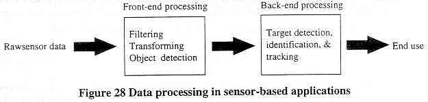
In front-end processing, the computational activities tend to be rather static, i.e. the same manipulation of the data is performed over and over again without great concern for the meaning or significance of the objects contained in the image. Front-end processing systems usually have two dominant concerns:
1. Keeping up with the flow of data from the sensors.
2. Providing the necessary computational performance in a package that meets the size, weight, and power constraints of the target platform (e.g. aircraft).
Keeping up with the flow of data from the sensors has two crucial components: throughput and latency. A sensor typically generates data at a rate that is a function of the number of bits used to represent each image or data sample and the rate at which samples are being taken. A basic requirement for a computing system is that it be able to process data at least as fast as it is generated. In addition, there are usually requirements for the maximum time a system is allowed to take to process a single image (the latency). The throughput can often be increased by, for example, increasing the number of processors at work. Doubling the number of processors may permit twice as many images to be processed in a given unit of time. Increasing throughput may not, however, improve the latency. Doubling the number of processors does nothing to increase the speed at which a single processor can finish processing a single image. In general, latency requirements present a more challenging problem to systems designers than do throughput requirements. Trends in front-end processing systems are discussed later in this section.
Back-end processing focuses on understanding the content of the image to identify and track targets. While such systems may be deployed on the same platform as the sensor, many processing systems today relay the output of the front-end processing system to a system closer to the end user. Consequently, back-end processing systems may not operate under the same size, weight, and power constraints as the front-end processing systems.
140
Synthetic Aperture Radar (SAR)
Synthetic aperture radar is a remote sensing technique used primarily to obtain high-resolution ground images from sensors flown on an aircraft, satellite, or other space vehicle. Unlike passive sensors which detect the reflected energy of sunlight or the thermal or microwave radiation emitted by the earth, SAR is an active sensor technique that generates pulses of electromagnetic waves toward the ground and processes the reflected echo signals. Consequently, SAR can be used day or night and under any weather conditions for a variety of civilian and military purposes in areas such as geology, agriculture, glaciology, military intelligence, etc. [84,85].
An on-going objective of SAR systems is to improve the system's resolution, defined as how well the system is able to distinguish between two closely spaced objects. In conventional radar systems, the resolution in the cross-track direction (perpendicular to the line of flight) is determined by the duration of a pulse. Shorter pulses (at the cost of greater energy requirements) give greater resolution. In the direction of the line of flight, resolution is limited by the size of the physical antenna and the operating frequency of the radar. Antenna theory dictates that an antenna several kilometers in length would be needed to resolve ground objects 25 meters in diameter [86]. Building an antenna of this size is not feasible. Synthetic aperture radar is a technique to improve the resolution of a radar system without increasing the size of the physical antenna by taking advantage of the motion of an air- or space-borne sensor. Figure 29 shows a standard SAR geometry. A small antenna travels in the direction of the line of flight, and emits short pulses of microwave energy across an area of earth, delineated by the dark lines, at a particular repetition rate. Each pulse will cause an echo pattern that will be captured as a matrix of data points.
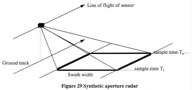
The sensor transmits pulses repeatedly as it passes by an area. Because of the sensor's motion, a given point target lies at different distances from the sensor for different pulses. Echoes at
141
different distances have varying degrees of "Doppler shift,"20 which can be measured. Integrating the individual pulse echoes over time creates an image.
Each energy pulse can result in a large number of data points. A typical image may consist of hundreds of thousands of samples, with each sample requiring 5-8 bytes of data [87]. Performing the necessary signal processing using discrete Fourier transforms (a widespread signal processing function) and matrix transformations may require several billion computational operations per second [86].
The reflections of these pulses are recorded and integrated together to achieve an effective antenna width equal to the distance traveled during the time period, and a maximum resolution in the direction of the line of flight equal to half the size of the physical airborne antenna. The resolution in the direction of the swath width (perpendicular to the line of flight) is proportional to the length of each microwave pulse such that shorted pulses should lead to better resolution. Since there are physical limits to how short the pulses can be and still generate useful echoes, a variety of complex techniques have been developed that employ pulses of varying frequencies to obtain high resolution [86].
| X-SAR sensor | RASSP SAR Benchmark |
|
| Date | 1993 | 1995 |
| Physical antenna size | 12.1 x 0.33 meters | |
| Nominal altitude | 250 km | 7.26 km |
| Frequency Band | 9.5 - 19 MHz | Ka-Band |
| Platform | Intel Paragon (various configurations) |
Intel Paragon (12 compute nodes) |
| Pulse repetition frequency | 1302 - 1860 pulses per second |
556 pulses per second |
| Sampling frequency | 11.25 - 11.5 million samples per second |
1.125 million samples per second |
Table 25 Mission parameters for X-band SAR sensors.
Sources: [87-89]
Table 25 illustrates some of the parameters for the X-band SAR sensor deployed by NASA on the Space Shuttle together with the Rapid Prototyping of Application Specific Signal Processors (RASSP) SAR benchmark developed by MIT Lincoln Labs and implemented on an Intel Paragon
_____________________
20 The Doppler effect is the change in frequency of a signal that results when the distance between a signal source and receiver are changing. The classic example is the drop in pitch (frequency) of a train whistle as a train passes a stationary observer.
142
at The MITRE Corp. [89,90]. The Spaceborne Imaging Radar-C/X-Band Synthetic Aperture Radar (SIR-C/X-SAR) was flown in two Space Shuttle missions in 1994 during which 4 Terabytes of data were collected and processed in subsequent years by various teams of researchers. Table 26 shows the time taken on an Intel Paragon to perform the correlation processing of data collected by the Space Shuttle's systems over a 20 second period. These results represented the first use of a commercial MPP systems to process high-volume SAR data in near real time [91].
| Paragon XP/S 35+ | |||
| No. channels of imaging data |
No. Nodes | CTP | Time (sec) |
| 1 | 64 | 2,621 Mtops | 36.0 |
| 4 | 256 | 7,315 Mtops | 49.0 |
| 8 | 512 | 13,235 Mtops | 55.0 |
Table 26 SIR-C/X-SAR processing times on the Intel Paragon. Source: [91].
The leading research done at the Jet Propulsion Laboratory has demonstrated high sustained performance on Grand Challenge SAR problems. In November 1997, investigators achieved over 10 Gflops sustained performance on a 512 processor Cray T3D (CTP approx. 32,000 Mtops). In 1998, investigators achieved 50 Gflops sustained performance on a Cray T3E with 512 nodes (CTP approx. 115,000 Mtops). Thus, only recently has commercial HPC technology been able to process SAR data at a rate that matches the data production of radar devices such as those flow on the Space Shuttle [92].
The RASSP SAR benchmark is an SAR image formation problem that has moderate computational and throughput requirements that are consistent with the requirements for some on-board real-time processing on unmanned aerial vehicles (UAV).
Traditionally, SAR computations have been performed by special-purpose, often customized, digital signal processing (DSP) hardware. Because of the size, weight, and power constraints, the systems have employed such exotic technologies as stackable memory units that permit a given amount of memory to be packaged in a smaller amount of space than is the norm.
There are two dominant trends in SAR hardware development. First, there is a great deal of pressure by procurers to use systems based on commercially available technologies. Second, the growing computational demands of SAR have fueled efforts to develop sizeable parallel processing platforms consisting of tens, or hundreds of processors.
In the efforts to move away from customized hardware solutions, two general approaches have been pursued. One approach has been to use general-purpose parallel processing systems, like the Intel Paragon, for front-end data processing. There have been a number of difficulties with this approach that have limited the use of general-purpose systems for such applications. While the systems have adequate computational capability, they tend to use processors that consume too
143
much power21, or employ packaging that does not make the best use of the space available. The two factors are often related. One of the advantages of physically separating components is that heat is more easily dissipated. Second, the architecture of general-purpose systems in many cases is poorly suited for signal processing applications. One example is the memory system architecture. To build general-purpose systems, system architects have gone through great pains to develop sophisticated cache systems. A fundamental assumption is that the instructions or data needed in the near future are likely to be those that were recently used. While this is true for many commercial and scientific applications, it is not true for image processing systems. Unrelenting real-time data streams continually present processors with new data. The overhead required to maintain the cache systems becomes a liability [93]. When general-purpose systems are used for signal processing applications, it is usually in non-embedded settings, such as those used to process the Shuttle's SIR-C/X-SAR data.
The alternative approach has been to utilize commercially available processors that have the best performance/power characteristics, and architect systems around them that are oriented towards the specific demands of signal processing applications. Besides having good size/power/weight parameters, advanced systems must have high-throughput/low-latency interconnects, and, preferably, the flexibility necessary to incorporate a mix of heterogeneous processors that will perform the computational tasks for which each is best suited. For example, Mercury Computing Systems, a market leader, has an architecture that permits low-power general-purpose processors such as the i860 and the PowerPC 603e to be integrated with digital signal processors such as the SHARC [94].
The companies that have emerged as leaders in the embedded systems market--Mercury Computing Systems, Sky Computers, CSPI, and Alacron--are not general-purpose systems vendors. Instead, they established themselves as providers of single-board accelerators employing one or more CPUs such as the i860 or specialized DSP processors and later expanded into multiboard systems with scalable interconnects. Because some of the fundamental algorithms of signal processing like the Fourier Transforms require a good deal of inter-node communication, these interconnects must have high throughput and low latency characteristics; conventional networking interconnects are not suitable. The resulting machines are called DSP multicomputers. Most of the DSP multi-computers are not particularly powerful in comparison with today's general-purpose systems. Table 27 shows two systems that have been deployed by Mercury within the last two years.
______________________
21 For example, Mercury Computer Systems, Inc., a leading vendor of embedded computing systems used the i860 (40 MHz), but did not use the i860 (50 MHz). The latter provided 25% better performance, but required three times as much power [ 18].
144
| Year | System | Usage | CTP |
| 1997 | Mercury Race (20 i860 processors, ruggedized) [95] |
SAR system aboard P3-C Orion maritime patrol aircraft |
866 |
| 1996 | Mercury Race (52 i860 processors) [96] |
Sonar system for Los Angeles class submarine |
1,773 |
Table 27 Signal Processing Systems sold by Mercury Computer Systems
In spite of their modest performance, the systems are quite controllable if one considers other qualities. First, the systems are rarely found as stand-alone systems; relocating these embedded systems would significantly hamper the function of their host system (i.e. submarine) and could hardly go unnoticed. Second, such systems have not been sold in great numbers outside of military customers, although Mercury is cultivating real-time embedded commercial markets such as video servers and hospital imaging systems. Even so, the configurations of the latter are significantly smaller than those listed above. Third, the systems deployed in military applications frequently have special qualities such as ruggedization not needed for stationary commercial systems.
Although many of the systems deployed in recent years have modest performance relative to commercial general-purpose systems, the performance has improved, and will continue to increase dramatically. First, the number of processors in a configuration has increased significantly. Until recently, systems employing more than a handful of processors were extremely rare. DSP multi-computers with 20 or more processors are now relatively mainstream systems. Second, as the embedded systems industry moves from the modest i860s (CTP 66.7 Mtops) to much more powerful PowerPC 603e (CTP 450 Mtops for the 200 MHz version), the performance of configurations will increase sharply. For example, in 1997, Mercury Computer Systems shipped a 140-processor system with a CTP of over 27,000 Mtops [94].
Space-Time Adaptive Processing Benchmark
Space-Time Adaptive Processing (STAP) is an advanced signal processing technique designed to improve the functional performance of airborne radar systems with little or no modification to the basic radar design. These techniques, employed after some standard pre-processing is performed on a signal, suppress the sidelobe clutter. STAP techniques adaptively combine samples from multiple signal channels and pulses to nullify clutter and interference. The algorithm takes the output of pre-processing and calculates and assigns different weightings to the results before recombining them into a final output. The term "adaptive" refers to the manner in which the algorithm adjusts the weightings in response to changing conditions in the signal environment.
STAP algorithms are highly computationally intensive and beyond the capabilities of most processors used in current airborne platforms [97]. However, they are likely to be important elements in the future as platforms are upgraded. Benchmarks run on available technologies provide some indication of the performance needed. One benchmark developed by the MITRE
145
Corporation and Rome Laboratories is RT_STAP, a benchmark for evaluating the application of scalable high-performance computers to real-time implementation of STAP techniques on embedded platforms [97]. The choice of system will necessarily be a function not only of performance, but also the size/weight/power/cost factors described above.
RT_STAP is based on the Multi-Channel Airborne Radar Measurements (MCARM) data collection system developed by Westinghouse for Rome Laboratory in the early 1990s. The system uses a 32-element antenna, transmitters, and receivers capable of generating L-band ( 1.3 Ghz) radar measurements. The 32 antenna outputs are combined to produce 22 channels. Generating signals with a pulse repetition rate of 250-2000 Khz and a pulse width of 50 to 100 microseconds, the system then records data at a sampling rate of 5 million samples per second [97].
The RT_STAP benchmark suite provides three tests of varying difficulty. The easiest benchmark, requiring a sustained throughput of 0.6 Gflops, reflects the computational demands of technology in current radar systems that perform a function similar to STAP. The medium and hard benchmarks, requiring sustained processing rates of 6.46 and 39.81 Gflops respectively, are more fully adaptive implementations of STAP and generally beyond the capabilities of widely deployed systems today.
The computational requirements are determined not only by the complexity of the algorithm used, but also by the overriding constraint that the throughput and latency of the system must be such that the system can process data at least as fast as the sensor can generate it. In the case of RT_STAP the system must process input data volumes of 245.8 thousand, 1.97 million, and 2.7 million samples with a maximum latency of 161.25 milliseconds for the easy, medium, and hard cases, respectively.
Figure 30 shows the performance of various configurations of the SGI Origin2000 on the RT_STAP benchmark. The dark solid line indicates the threshold at which a configuration is able to process the necessary data within the 161.25 millisecond latency limit.
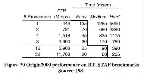
The benchmarks illustrate a number of points. First, a single R10000 processor has sufficient performance to perform the kinds of clutter cancellation functions used in current radar systems
146
(easy case) Second. the requirements of the medium benchmark exceed the performance of a deskside Origin2000 (8-processor maximum). Third, the hard. or fully adaptive STAP algorithm exceeds the capability of even a 32 processor (two-rack) Origin2000.
Of course, the space/weight/power constraints of actual airborne platforms are likely to preclude the Origin2000. Nevertheless, the benchmarks give all indication of the minimum performance requirements necessary for STAP algorithms of varying complexity.
Summary and Conclusions
Forces Modeling and Simulation
Simulation is playing an increasingly important training role in DoD. The U.S. military is placing great emphasis on virtual environments for training in and analysis of combat operations. There are three types of simulations in use: live, virtual, and constructive. Live simulations replace sensor information with computer data feeds. The simulated sensor readings are correlated with physical cues to match as closely as possible what the warrior would actually experience. The classic example of live simulation is a flight simulator, where the pilot manipulates the controls and the simulation adjusts the pilot's view and his instruments. Virtual simulation puts the simulator into a scenario with other entities; i.e., a tank crew will interact with other tanks in a realistic scenario. Some of the other tanks will also be crewed by soldiers; others will be computer-generated entities. Both live and virtual simulations are characterized by the participation of the man-in-the-loop; i.e., the trainee operating his vehicle or aircraft.
147
The third category, constructive simulation, has no man-in-the-loop feature.
Instead, the battles are fought with no or minimal human intervention. Computer
generated forces (CGF) are used to populate the battlefield. Commanders are
able to control units, or the computer can control the units. CGF's were
initially invented to allow tank crews to have an opponent. The 14 crews
that make up a tank company would each be in their own simulator CGF's would
represent the enemy tanks in the scenario. This removed the need to construct
and man simulators for the enemy forces [99].
History
Simulator Network (Simnet) was the first system to support all three types of simulation. It was developed in the mid-80's in a DARPA funded project. The information needed for the simulation is sent over local or wide-area networks, allowing widely dispersed simulators to participate. Simnet, however, suffered from several limitations:
The work to extend Simnet has led to the Distributed Interactive System (DIS) protocol, and associated IEEE standard (1278) which has specifications for more vehicle and weapon types and non-visual effects [99]. The DIS standard, however, is still limited in that it does not allow all simulations to interact. As a result, a new distributed architecture, High Level Architecture (HLA), was adopted in October 1996. HLA is designed to support heterogeneous hardware and software, multiple independently designed sub-architectures, simulations distributed over local- and wide-area networks, and 3D synthetic terrain environments and databases.
More critically, HLA addresses interoperability among the different levels of command that may be represented in a simulation. These levels can range from the individual weapon system, through platoon, company, battalions, etc. HLA treats these as aggregates. For example, a company is represented as three platoon entities and one commander entity [100].
In 1994, the first large, real-time simulated exercise was held: Synthetic Theater of War - Europe (STOW-E). The exercise used Simnet and DIS protocols, CGF's, and man-in-the-loop simulators from all the services. Wide-area networks and a transatlantic link connected 14 U.S. and European sites. Over 2,000 entities, most computer-generated, were involved [99]. The 1995 Engineering Demonstration (ED- lA) exercise increased the number of entities to 5,371 vehicles hosted at 12 sites in the continental US. [101].
Current state
Typical training installations will have a set of simulators for the type of unit(s) training there. For example, an Army installation might have a collection of M-1 or Bradley simulators. The Marine Corps is developing simulators for individual soldiers to train as small teams. These
simulators can be used singly. with all other entities portrayed by CGF s. Or, the simulators might be combined for small unit training with only the "enemy" represented by CGF's.
CGF entities have four main components: action, perception, fatigue (physical fatigue for a soldier, or fuel and engine state of a vehicle), and damage. A single simulator, such as a tank, typically uses a PC or workstation class machine. By comparison, a single workstation is capable of generating several dozen CGF's or more for a simulation. The more detailed and "realistic" the CGF's, the fewer that can be hosted on a single machine due to the computational requirements.
As an example, the Chemical Biological Defense Command (CBDCOM) has developed a set of simulators for the Fox CBD vehicle. The simulations include the Fox vehicle itself, the MM1 detector, the M21 standoff detector, and the LSCAD, a lightweight version of the M21. They have also designed threat scenarios, such as a missile attack that releases a gas cloud along the front of an advancing armored formation.
These simulation tools have been used to evaluate improvements to existing equipment and newly designed equipment. These simulated evaluations have allowed designers the luxury of trying a number of ideas without the expense of building multiple prototypes. The simulations also provide the opportunity to develop tactics for the use of new equipment while it is still in development. Thus, when the equipment becomes available in quantity, the tactics for its use are already in place.
The computing equipment used at CBDCOM to participate in a simulated exercise includes PC' s (under 500 Mtops) for the MM 1 and M2 1 detectors. Three SGI Onyxes are employed for:
The largest Onyx is a four-processor system (625 Mtops). The Onyx's are used primarily for their interactive graphics capability, not number crunching [102].
The mix of machines at CBDCOM is typical of most installations. The system is expressly designed to be a cost-effective system. This requires the use of commodity, off-the-shelf computing equipment.
Large-scale forces modeling
Modular Semi-Automated Forces (ModSAF) projects support the simulation of large-scale military exercises. Unlike the simulations described in the previous section, these do not normally involve man-in-the-loop simulators. Instead, the purpose is to allow commanders to examine large-scale tactics and to analyze the results of various tactical and even strategic decisions.
Nominally, it is possible to add entities to the standard DIS simulation, by adding more workstations, each modeling some number of CGF's. However, the DIS standard is not that
149
scalable. First, broadcast messages can overwhelm the networks as the number of entities increases. Second, the number of incoming messages can exceed the processing capabilities of the individual workstations. Much work in the ModSAF community is focused on solving these problems.
The Synthetic Forces Express (SF Express) project is exploring the utility of using parallel processors, both large MPP's and smaller clustered systems, in conjunction with intelligent data management as a solution to the communications bottlenecks. The project is a collaborative effort among Caltech's Center for Advanced Computing Research, the Jet Propulsion Laboratory, and the Space and Naval Warfare Systems Center San Diego.
The general approach is to use "interest management" [103] . Essentially, entities in the simulation state the events they are interested in. Messages go only to those entities interested in that message. This allows, for example, a vehicle to be interested in other vehicles within a certain range, or that are within some specific physical area, such as a canyon, town, etc. Once the interests have been stated, the vehicle is no longer informed of vehicles/entities that do not match those interests. A vehicle's region of interest is dynamic and changes as that vehicle moves on the terrain database during the simulation.
The communications architecture uses a primary router node to handle communications for a cluster of standard simulation nodes, as shown in Figure 31. The simulation nodes are typically a subset of the processing nodes available on an MPP, or nodes in a PC cluster. Each simulation node talks to the router, rather than broadcasting its information, as is the case in the standard DIS simulation. A simulation node will have one to several dozen CGF's on it. Each CGF will declare its interests~ at the start of the simulation and during the simulation as those interests change. The node will forward the union of the interests of its CGF's to the primary router. The primary router will collect all messages from its cluster of simulation nodes and forward to the simulation nodes only those messages that match each node's interests. Experiment has shown that one primary router can handle the communications and interest declarations for a cluster of simulation nodes that models a total of one to two thousand vehicles.
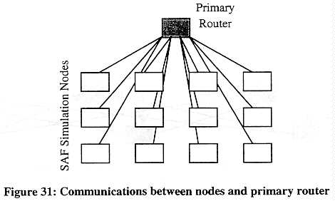
150
When the simulation scales beyond the capabilities of a single primary router node, additional nodes can be allocated to create new clusters, each with its own primary router node. At this point, two additional communication nodes are needed for each cluster as shown in Figure 32. The pop-up router (labeled U) handles the out-going messages from the primary router. The pulldown router (labeled D) collects the interest declarations from the primary router and uses these to determine which messages in the pull-down layer are to be delivered to the primary router. This communications architecture is scalable and handles a variety of machines. Simulation nodes can be a single processor workstation, or a node in an MPP-class machine. The routers are similar: each could be a single processor workstation, or a node in an MPP-class machine.
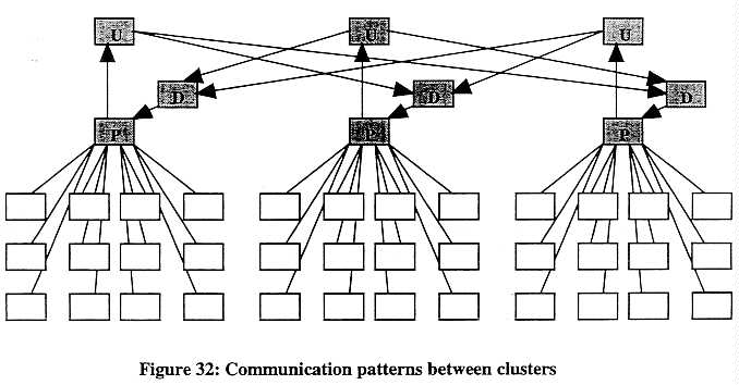
A variety of tests have been conducted. They include tests on a single MPP host. on a cluster of workstations, and on multiple, geographically distributed MPP's. These tests are summarized in Table 28 [101].
151
test |
machine |
nodes |
CTP |
vehicles |
entities |
| single MPP | ORNL Paragon | 360 |
9626 |
5,713 |
6,697 |
680 |
16737 |
10,913 |
13,222 |
||
1024 |
24520 |
16,606 |
20,290 |
||
| 6 MPP's, June 97, 2 hr simulation |
Caltech HP Exemplar |
256 |
60345 |
13,905 |
|
| ORNL Paragon | 1024 |
24520 |
16,995 |
||
| NASA Ames SP-2 | 139 |
14057 |
5,464 |
||
| CEWES SP-2 | 229 |
21506 |
9,739 |
||
| Maui SP-2 | 128 |
13147 |
5,086 |
||
| Convex HP Exemplar | 128 |
34425 |
5,348 |
||
| cluster | two Beowulf systems |
80 |
3,000 |
Table 28: Synthetic forces experiments
A 50,000-vehicle simulation was also demonstrated at SC97 in November 1997. A 100,000vehicle simulation was completed on March 16, 1998 involving 13 heterogeneous MPP's at 9 different sites [104]. Work is now being directed toward enriching the simulation environment. The current terrain database used for the simulations is a desert terrain with relatively few features. In addition to using more feature-rich terrain databases, work is proceeding on incorporating improved weather effects and such weather-related effects as gas clouds, smoke, etc. It is estimated that a simulation node that can support x vehicles in the current desert terrain will be able to support one-half x in a more complex terrain [105].
Conclusions
The preceding discussion leads to the following conclusions:
Littoral Warfare
Littoral warfare refers to military operations in littoral, or coastal, areas of the world. This type of warfare has a particular impact on naval operations, and imposes some difficulties on air
152
operations as well Particularly with the end of the Cold War. the U S Navy has become more concerned with operations in littoral seas.
The need to operate in littoral areas imposes requirements that demand high performance computing Some of these applications have already been covered in this report They include submarine maneuvers in shallow waters (see Submarine design, page 101), and regional weather forecasts (see Modeling coastal waters and littoral seas, page 87) Two additional areas are examined briefly in this section electronic warfare and surveillance.
Electronic warfare [106]
Traditional electronic warfare (EW) for the Navy has been in the open ocean, an environment that is relatively easy to manage. The open ocean provides less interference with propagation than land In the current world situation, however, the Navy needs to operate closer to land, and has taken on the task of providing EW support for inland forces.
The electronic database of the past has been one that contains an estimated order of battle for the opposing forces. The database was relatively static and based on archival information. The estimates of radar and EW effectiveness were limited to simplistic coverage zones as a function of altitude and range. Tactical maps were produced from this data by simply penciling in the location of an emitter and its coverage.
Simulations that involved, for example, tracking a missile in its flight over the ocean were relatively easy, since the environment was sparse. Tracking that same missile over land is considerably harder. High performance computing has been particularly useful during the research phase of such projects. The assumption is not that a ship will have cutting edge computing. Instead, the researchers use the high performance computers to develop the algorithms and determine what environmental factors are significant and which are not. By the time the code is developed and the environmental factors have been reduced to only those that are significant, the code is expected to perform well on the computing platforms that will then be available in the fleet.
Parallel versions of the current codes have been developed, primarily for shared memory parallel systems such as the SGI PowerChallenge and Onyx systems. These are coarse grain parallel codes, deriving the parallelism over the target's bearing angle or aspect angle. A vendor's parallel tool will often not be suitable, as it attempts to parallelize the inner as well as the outer loops. This forces the programmer to "fix" what the auto-parallelizer has done.
The Navy is working on a new, integrated EW system. It will use current intelligence estimates of the opposing force's electronics capabilities, and integrate terrain information and weather into the estimates of electronic coverage. The EW assessments can be displayed on screens that show locations of friendly forces and geographic information. Bringing this data together is primarily a network and communication bandwidth problem, not a computing problem. The integration of the data into a useful tool for the on-scene commander, however, is a computing problem.
The Naval Research Laboratory is developing the tools needed to integrate the various EW information streams into an integrated product. They are developing adaptive techniques that will
153
select from a range of fidelities The choices will be based on the information available intelligence estimates, environmental data (weather, sea state, etc ), terrain data, force dispositions, and the time available to compute a solution
Surveillance [107]
The Advanced Virtual Intelligence Surveillance Reconnaissance (ADVISR) program is developing an integrated system of underwater, surface, airborne, and space-borne surveillance sensors. The project is using high performance computing in three ways.
The first way involves simulation to model the performance of the sensors The current program, for example, is designing underwater sensors that will rest on the continental shelf off a coastline, with potentially hundreds of sensors involved in an actual deployment The sensors will communicate with a master sensor that can then be queried by friendly forces for information. Simulation is being used in two orthogonal directions. First, an individual sensor on a workbench can be wired into the simulation. The simulation provides all the inputs that the sensor would "hear" if it were in the water off a targeted coast. The sensor then performs its built-in analysis functions. When it needs to communicate with the master sensor or other sensors in the array, it does so. The simulation then handles the other side of such conversations. This allows the researchers to test the sensor in the lab, make changes, retest, etc. without having to actually deploy the sensor in the ocean each time. The second orthogonal use of simulation is modeling a large number of such sensors. This level of simulation requires that each sensor be represented in the simulation. Since there would be up to several hundred such sensors deployed, the simulation must represent each of these, its inputs, its evaluations, and its communications. Currently, this level of simulation is being performed on the 336-node Intel Paragon located at the Space and Naval Warfare Systems Command (SSC) in San Diego.
The second use of high performance computing in this project occurs in the visualization area. The researchers are developing a virtual world that will allow tactical commanders to view their environment. The virtual world will incorporate both land and underwater topography, locations of friendly, hostile, and neutral forces on land and sea, the locations of deployed sensors, and various environmental factors including weather patterns. The virtual world is under being used in two ways. The first is to test the sensors themselves. Objects such as submarines, schools of fish, etc., can be placed in the virtual world. The simulation described above is then used to determine how well the sensors can detect the objects. The second use for the virtual world is to experiment with techniques for displaying this information to tactical commanders. The virtual world currently requires two multi-processor SGI Onyx systems.
The third use of high performance computing in this project is to integrate the results of all the sensors to produce the inputs to the virtual world. The goal is to reduce the volume of information coming from sensors to a useable level that commanders can assimilate without leaving out critical information. This requires not only the collection of the information, but a decision-making process that prioritizes the information before sending it to the display system. This integration of information is being developed and tested on the Intel Paragon at SSC. Thus, it currently requires a level of computing beyond that normally found in fleet flagships. It is
154
anticipated that the level of computing in the fleet will improve with developments in the computer industry before the system is ready for deployment. The final level of computing needed will likely be less due to algorithmic improvements in the software and decisions as to which information streams ultimately will prove useful and which can be left out of the final product.
Summary
Littoral warfare research and development currently have high computational demands. While these demands will be somewhat less by the time the systems are deployed, an implicit assumption is that better shipboard and airborne computing platforms will be available. High performance computing is allowing the research and simulation of the future systems to take place today, so that the software will be in place when the new hardware arrives.
Nuclear Applications
Introduction
The development of nuclear weapons involves the study of physical phenomena in the extreme. The phenomena are highly non-linear, often in non-equilibrium, and frequently on time- and space-scales that are very difficult to measure and interpret empirically. Furthermore, the development process is multi-disciplinary, involving studies of kinetics, fluid dynamics, structures, complex chemical reactions, radiation transfer, neutron transfer, etc. [108]. Since the mid-1960s, computer programs have been developed to try to model these complex processes. Nuclear weapon development and maintenance uses dozens of different codes that represent various pieces of this complex phenomenon.
Evolution
The earliest nuclear weapons were developed using hand-operated calculators. After the dawn of the computer age, however, the national laboratories were often the first users of new systems from such companies as Control Data Corporation, Cray Research, Thinking Machines, and others. As early adopters they were willing to accommodate a good deal of pain in dealing with immature hardware and software platforms for the sake of the obtaining the highest levels of computing power available. The development of nuclear weapons and advances in supercomputers were closely linked throughout the 1970s and 1980s.
The evolution of the computations and the computers to support them fall, very roughly, into three phases, corresponding to one-dimensional, two-dimensional, and three-dimensional computation.
The early weapons employed single, simple primaries (detonation devices) whose behavior could be satisfactorily modeled using one-dimensional computations. Such computations required on the order of only a single megabyte of main memory and were performed on machines such as
155
the CDC 7600 and Cray-1S (CTP: 195) During the 1970s, these machines were used to carry out two-dimensional computations, albeit at under-resolved resolutions and less than full physics.
During the 1980s, with the introduction of the Cray X-MP and. later, the Cray Y-MP, two-dimensional modeling with well resolved, full physics became common. Two-dimensional computations were done on single processors of the Cray XMP (CTP: approx. 350 Mtops) and Cray YMP (CTP: 500). Production runs on more than one processor were uncommon, because multi-processor jobs used CPU cycles less efficiently than did multiple jobs running on individual processors. Over time, two-dimensional codes were improved. Resolutions were increased, approximations needed to simplify code and reduce computational requirements were improved, and codes were enhanced to include a more complete set of physics and chemical models. Many production codes continue to be 2D codes. The 1980s also saw the first three-dimensional, under-resolved, reduced physics computations.
During the mid-1990s, the objective of computational research shifted from weapons development to stockpile maintenance. The questions asked were no longer, "how can we build a new device with a higher yield that will fit into a smaller container and survive more hostile environmental conditions?" Rather, research was oriented towards understanding, for example, the affects of aging on the ability of an existing device to function as designed. Many of these non-normal phenomena are, unlike detonation phenomena, inherently three-dimensional. They include [109, 110]
1. the effects of microscopic fractures;
2. chemical changes such as polymer breakdown, metal corrosion, and debonding;
3. physics processes related to fissure analysis and stability;
4. the operation of physical devices with parts moving in three dimensions.
The shift from 2D modeling to 3D modeling requires an enormous jump in computational capability. Not only does a third dimension compound the number of grid-points, it also requires greater numbers of variables per grid-point and, as the resolution of grids increases, smaller timesteps. While the 3D under resolved, reduced physics modeling codes can execute on a Cray YMP, this system does not have the memory necessary to execute a model that is sufficiently precise and accurate to be useful. In the United States, the Intel Paragon was the first machine with a large enough memory (32 Gbytes) to run credible 3D resolution reduced physics simulations. This system, which represents a hundred-fold increase in CTP value over the single processor Cray YMP, is considered a minimum for credible 3D simulation. Systems with ten times more power (1000x over a Cray YMP, or 500,000 Mtops) are considered suitable for a broad range of 3D simulations in this application domain. Full physics 3D modeling requires at least an order or two of magnitude more.
Gaining confidence
In each of these cases, the principle objective was not only to build a device, but also to have a certain assurance, or confidence, that the device would function as intended. Unlike mechanical
156
devices like airplanes in which a single unit can be tested, modified, and certified before being used by a customer, nuclear devices either work or they do not. There is no opportunity for in-the-field modification to correct an error. Gaining confidence in a device can be done in two ways. The traditional way is to build a device and test (explode) it; if the test is successful, then build several more devices just like it and assume that these copies will behave as the original. As computational methods and capabilities have advanced, simulations of physical processes are increasingly able to model the behavior of a particular device under particular circumstances.
The confidence one can place in the results of the simulation is directly related to (a) the extent to which a code has been validated, and (b) the extent to which the phenomenon being simulated is similar to the phenomena against which the code was validated. Validation consists of running a simulation of a test that has been carried out and verifying that the computed results are acceptably close to the empirical results. If a validated code is used to model small variations on a proven design (e.g. replacing one small component with another one substantially similar to it), then practitioners have a great deal of confidence in the computed results. The more the simulated situation differs from established practice, the more computing power is needed for the simulation, and the less confidence one has in the computed results. In general, one will have rather little confidence in computed results alone for a simulation of a new weapons design concept, or a phenomenon that has not occurred during actual testing. A researcher with a high-performance computing system but inadequate test data has been compared with a drunk driving a car: the more the drunk has to drink the better he thinks he drives. Comparably, with just a high performance computing system a researcher may obtain impressive results, but have no way of knowing whether those results match reality [111].
Greater amounts of simulation with higher spatial resolution and physics fidelity may not give full confidence, but they may help developers determine which tests will be most beneficial in the development process. The net result may be fewer (but not zero) tests, at lower costs, in shorter timeframes.
Confidence in computational results is gained in a number of ways as testing and experience grow [109].
1. The underlying physics models. Today, there is great confidence that the underlying physics models used in many areas of nuclear investigation are correct. These models accurately reflect the nature of the world and are quite stable. Moreover, these models are available and understood by scientists throughout the world. Needless to say, there are many fields (e.g. three-dimensional compressible flow) in which the understanding and ability to model physical phenomena precisely are lacking.
2. The numerical methods. The nature of the problem dictates the resolution, which dictates the computational requirements. If the machine being used is not able to offer the necessary memory and CPU cycles, then one will have little confidence in the results, even if the numerical methods and algorithms are themselves sound.
3. The fidelity of the computation. Does the code actually model the real world? Code must be validated against empirical tests. Many of the phenomena modeled in weapons development
157
or maintenance are not explicitly nuclear. To validate these parts of the code, non-nuclear test data can be used. In many (but not all) cases, such data is available internationally.
4. Finally. there are parts of the code that model the highly non-linear effects of the nuclear explosion itself. These codes can be validated only with nuclear test data.
Of these four elements, only the second is directly affected by export control of hardware. To have full confidence, however, all four elements must be available. The implication is that advanced hardware by itself contributes little to the development or maintenance of nuclear devices; in conjunction with nuclear and non-nuclear test data, however, computing may be quite beneficial.
When test data are available, incremental increases in computing power provide incremental benefit. Practitioners are able to run bigger problems, improve the resolution of codes, refine approximations, use improved physics models, reduce the turnaround time, or do a combination of all of these [64,109,112]. This relationship is shown in Figure 33. The figure is not drawn to scale.

Computing Platforms and Nuclear Applications
Parallel computation is a maturing discipline within the nuclear weapons community. During the late l980s and early l990s, the Department of Energy national laboratories decided to step off the upgrade path offered by Cray Research's family of vector pipelined machines. Since the early years of this decade, the labs have invested a great deal of effort understanding and developing
158
parallel code. Today, many--but by no means all--codes are in their second or third generation on parallel platforms. Today parallel platforms are the principal production systems; few vector-pipelined systems remain in use at the National Labs.
Not only have production codes been ported to parallel platforms, they have been ported in a manner that makes porting to any other platform a relatively straightforward task. By using standard message-passing interfaces like MPI and writing code so that the heart of the application is shielded from the details of message-passing, code developers have limited to a small fraction the total amount of code that needs to be changed. While the development of a code might have required initially l5-20 person-years of effort, at Sandia porting the main production codes to parallel platforms required only 1-2 person years of effort per code. However, a good deal of work typically needs to be done to gain optimal performance on a particular platform.
Most of the production codes run and scale well on parallel platforms. Many codes, Monte Carlo calculations in particular, employ coarse-grain parallelism. These codes perform a large amount of computation relative to inter-node communication and are therefore relatively latency tolerant. Other codes, or portions of codes, are not as latency tolerant. These include several important physics packages and perhaps the deterministic particle transport codes, such as that represented by the SWEEP3D benchmark [113,114]. Wasserman, et al have compared the performance of two SGI systems employing the same microprocessor: the PowerChallenge and the Origin2000 [113]. They show that the improved latency-hiding memory systems of the Origin2000 have a substantial impact on the performance of benchmarks characterizing Los Alamos National Laboratory' s nuclear applications workload. Detailed analysis of which codes are likely to benefit most from high-performance interconnects is a subject of on-going research.
Trends for the future
There is no shortage of exceedingly demanding applications within the nuclear weapons community. Although it has been on-line for only a year, the ASCI Red system at Sandia National Laboratory has already been run at capacity by one application: CTH. Researchers have outlined a dozen applications ranging from the modeling of multi-burst ground shock (effects against deeply buried structures) to the simulation of neutron generator standoff that require a Teraflop or more of sustained performance, and 100 Gbytes to multiple Terabytes of main memory. These requirements significantly exceed the capabilities of the 250,000 Mtops configuration available to a single application today.22
The major shift anticipated by the ASCI program is use of 3D simulations based on first principles physics modeling [110]. Such simulations do not rely on empirical data to establish the initial and boundary conditions and macro-level approximations during a computational run. Instead, they model the activity of nuclear particles directly, subject to the fundamental laws of
____________________
22 The full configuration ASCI Red has over 4,500 compute nodes (CTP approx. 300,000 Mtops). Only about 3500 are available for a single application however. The machine has an unclassified portion and a classified portion. A given application will use one or the other, but never both at the same time.
159
physics. Table 29 shows ASCI projections of the computing requirements for 3D simulations based on first principles.
| Simulation | Teraflops required | Terabytes required |
| radiation transport | 123 Tflops | 40 Tbytes |
| shock waves propagating through explosive components |
150 Tflops | 75 Tbytes |
| chemical changes (polymer breakdown, metal corrosion, debonding) for highly localized phenomena |
30 Tflops | 5.5 Tbytes |
| detailed engineering simulations of microscopic degradation | 100 Tflops | 100 Tbytes |
Table 29 Computing requirements for first-principles simulations.
Source: [110].
Summary and Conclusions
Table 30 illustrates the computational power used in the United States to run various nuclear weapons development and maintenance applications.
| Machine | Year | CTP | Time | Problem |
| Cray-1S | early 1980s | 195 | 117.2 CPU sec | LANL Hydrodynamics code 1 |
| Cray-1S | early 1980s | 195 | 4547.1 CPU sec | LANL Hydrodynamics code 2 |
| Cray-1S | early 1980s | 195 | 1127.5 CPU sec | LANL Hydrodynamics code 3 |
| Cray X-MP/1 | mid 1980s | 316 | seconds | 2D, reduced physics simulation |
| Cray X-MP/1 | late 1980s | 500 | 1000's of hours | 1D, full physics simulation |
| Cray X-MP/1 | late 1980s | 500 | overnight | 2D, almost full physics (e.g. Monte Carlo neutron transport) |
| Cray X-MP/1 | 500 | overnight | 2D, reduced physics simulations | |
| 1995 | 1400 | Credible 1D and 2D simulations | ||
| Intel Paragon | 1994 | 46,000 | overnight | 3D reduced physics simulation of transient dynamics of nuclear weapon |
| ASCI++ | ?? | 50,000,000+ | days | First principles 3D modeling |
Table 30: Nuclear weapons related applications. Sources: [115,116]
Table 30 and the preceding discussion, lead to the following principle conclusions:
160
Cryptographic Applications
Cryptographic applications are those involved with the design and implementation of security codes, and the attempt to "break" codes to be able to read the encoded message. The historical experiences from World War II of the Ultra project in England to decode the German ciphers, and the similar project in the U.S. regarding the Japanese codes, gave the Allies significant military advantages.
The advent of parallel systems, be they low-end clusters or high-end massively parallel systems, has made it possible to break selective codes. The problem space is essentially divided across the available platforms, and each machine works on its portion, looking for a plain text result. Thus, it is possible using uncontrollable technology to acquire an ability to decipher messages.
However, being able to decipher a single message, or determine one key, does not necessarily imply an ability to read all the messages of one's adversary. There are two problems that must be solved if one needs a more complete ability to read messages encoded using a wide variety of keys. The first is a real time issue: decoding the message weeks after an event may be of no use.
161
The second is a volume issue: a single message may not be useful without the context of other messages on the topic Thus. there is a quantitative difference between the ability to determine a single key, and being able to read in real time all of an adversary's message traffic.
We have had extensive discussions with the intelligence community about cryptographic applications. While we cannot discuss directly the details of those conversations, we can make the following conclusions:
Problems with vector to MPP transition [117]
The cryptographic community has had the luxury of significant input into the design of the vector processor, in particular those manufactured by Cray Research. The advent of MPP platforms, and their dependence on general-purpose processors has greatly reduced this influence. The market for the MPP platforms is much larger than the scientific community alone, and is driven by commercial needs.
For cryptographic applications, the vector turns out not to be the primary advantage of the pipelined vector supercomputer (PVP). Instead, it is the high performance of the complete system that is important. The attention paid to the performance of each of the subsystems on the Cray vector machines does not (as yet at least) have a corollary in the MPP architectures.
First among the concerns is memory, both in size and in bandwidth. The MPP platforms offer larger memories than vector systems today. The bandwidth, however, is not adequate. This has been evident in other applications described in this paper, and cryptographic applications are no exception. Worse, they have a requirement for random access to memory. The cache performance of microprocessors is predicated on the assumption of locality of access. The cost to load a whole cache line when only one value is needed, and the use on some systems of write-through caches, lead to poor performance. Cache coherence protocols can actually make a series of random remote accesses worse. Finally, microprocessors generally provide no way to by-pass the use of the cache.
Second, cryptographic applications are primarily integer, not floating-point, codes. Less than 5% of operations in typical applications are floating-point codes. PVP machines exhibit excellent performance on either integer or floating-point operations. Microprocessors, on the other hand, give much better performance on floating-point than on integer operations. Two reasons account for this. First, the microprocessor integer unit is not distinct from the control logic. The system optimizes for the control logic, leaving the integer performance less than optimal. Second, the split between floating-point and integer operations affects the number of registers available to
162
each. For applications that are nearly exclusively integer, this means that half the register set is unavailable.
Some special operations are available in PVP systems as a result of lobbying by the cryptographic community. They would very much like to see some or all of these in microprocessors. These include:
The hardware vendors are aware of the desire for similar operations in today's commodity processors. However, very few are even considering adding the instructions. If these or other operations were added, it is necessary that they be accessible from high-level languages. The compiler does not have to be able to recognize when to use the instruction, but compiler directives or direct assembly commands should be available to the programmer. This is a productivity requirement given the need to develop all software in-house rather than take advantage of third-party software.
The last point is a combined system issue: ease of use. The MPP market has been very volatile, with new systems appearing that have at best limited connection to previous systems, and system software that is not retro-fitted to earlier systems. This places a tremendous burden on the application developers, both in the learning curve and in the actual hours committed to developing and maintaining code. This is not a problem unique to cryptographic applications. What makes it harder for this community, however, is the complete lack of third-party solutions. They cannot rely on a set of companies to provide updated software to match new computer systems.
Summary
Application characteristics
There is a wide range of applications that are of national security concern and that require high-levels of computing performance; thus, satisfying one of the three legs on which the HPC export control policy rests. The following features characterize the national security nature of the applications described in this report:
163
The applications can also be characterized by the computing requirements that make them doable on high-performance systems, but not doable in a useable form on lesser computing platforms:
Application bands
Figure 34 shows a histogram of the specific applications studied for this report. Among applications that require high computing levels, the bulk of them fall in the 15,000 to 25,000 Mtops range, primarily because this represents the performance of systems that have been available to researches over the past few years. As newer systems with increased performance come on line over the next one to two years, there will be an increasing number of applications that will appear in the 30,000 and up ranges. These will fall into two categories:
164
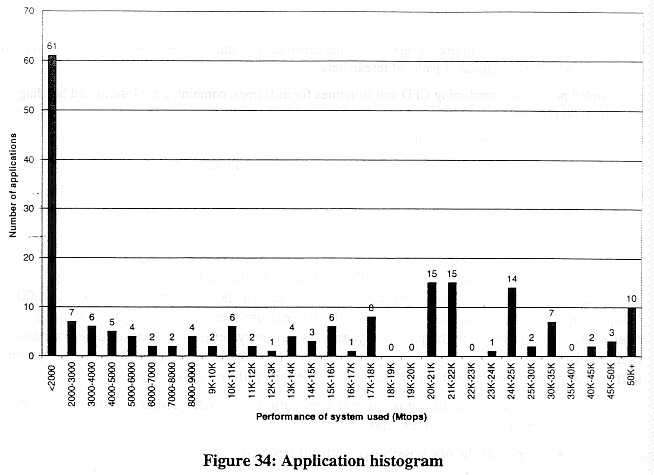
Looking more closely at performance levels of interest to policy makers, Table 3l shows applications in the 5,000 to 10,000 Mtops range. These represent CFD applications that examine specific parts of an aircraft or simple geometric shapes, moderate-sized computational chemistry problems, brigade-level battle simulations, and coarse-grain weather forecast models. The weather forecast models at this level are not accurate very far into the future. A significant implication is that such forecasts would not be suitable inputs to regional forecasts over an area of concern to military planners.
165
| CTP | CTA | Problem |
| 5375 | CFD | Modeling of flow around a smooth ellipsoid submarine. Turbulent flow,
fixed angle of attack |
| 6300 | CFD | Helicopter blade structural optimization code, gradient-based optimization
technique to measure performance changes as each design variable is varied. |
| 6332 | CWO | CCM2, Community Climate Model, T42 |
| 7100 | CFD | Helicopter rotor free-wake model, high-order vortex element and wake relaxation |
| 7315 | CFD | Particle simulation interacting through the standard pair-wise 6-12 Lennard-Jones potential, 50M |
| 8000 | CEA | Bottom contour modeling for submarine design |
| 9510 | CFD | Large-Eddy simulation at high Reynolds number |
| 9626 | FMS | 5.7K vehicle battle simulation |
Table 31: Applications between 5,000 and 10,000 Mtops
The next set of applications is shown in Table 32. These include simple radar cross-section problems, computational chemistry problems of increasing size, and operational weather forecast models. The weather forecast models are clustered just above l0,000 Mtops. These represent operational forecast models used by Fleet Numerical (and others) starting about 1995. While Fleet Numerical has since upgraded to more capable computers, this band represents a region of useable computing performance for weather forecasts. Global forecasts at this level of accuracy begin to be useful as inputs to regional forecasts. Computing power beyond this level allows global forecasts that are accurate further into the future.
| CTP | CTA | Problem |
| 10056 | CEA | Radar cross section of perfectly conducting sphere, wave number 20 |
| 10457 | CCM | Determination of structure of Eglin-C molecular system |
| 10625 | CWO | Global atmospheric forecast, Fleet Numerical operational run (circa 1995) |
| 11768 | CWO | SC-MICOM, global ocean forecast, two-tier communication pattern |
| 13004 | CCM | Particle simulation interacting through the standard pair-wise 6-12
Lennard-Jones potential, 100M |
| 13236 | CCM | Molecular dynamics of SiO2 system, 4.2M |
| 14200 | CWO | PCCM2, Parallel CCM2, T42 |
Table 32: Applications between 10,000 and 15,000 Mtops
Applications in the next range fall into two bands, as shown in Table 33. The first band is near l5,000 Mtops and the second is around 17,000 Mtops. At this level, available computers do not
166
uniformly fill the CTP range; thus. applications begin to "clump" around the CTP of specific machines. This range includes more accurate weather forecast models. simple explosion-building simulations, divisional-size battlefield simulations, and CFD problems that begin to model complete airframes of small objects such as missiles with some turbulent effects.
| CTP | CTA | Problem |
| 15976 | CWO | AGCM, Atmospheric General Circulation Model |
| 15875 | CSM | Water over C4 explosive in container above wet sand, building at a distance |
| 15875 | CSM | Water over C4 explosive in container above wet sand, alternate scenario
- container next to building, finite element |
| 15875 | CWO | Global atmospheric forecast, Fleet Numerical operational run (circa 1997) |
| 16737 | FMS | 11K vehicle battle simulation |
| 17503 | CCM | MD simulation using short-range forces model applied to 3D configuration of liquid near solid state point, 100K & 1M & 5M particles |
| 17503 | CFD | Aerodynamics of missile at Mach 2.5, 14-degrees angle of attack for laminar and turbulent viscous effects |
| 17503 | CFD | Large-Eddy simulation at high Reynolds number |
| 17503 | CWO | ARPS, Advanced Regional Prediction System, v 4.0, fine scale forecast |
| 17503 | CWO | Global weather forecasting model, National Meteorological Center, T170 |
| 17503 | CWO | AGCM, Atmospheric General Circulation Model |
Table 33: Applications between 15,000 and 20,000 Mtops
References
[1] Goodman, S. E., P. Wolcott, and G. Burkhart, Building on the Basics: An Examination of High-Performance Computing Export Control Policy in the 1990s, Center for International Security and Arms Control, Stanford University, Stanford, CA, 1995.
[2] Sunderam, V. S., "PVM: A framework for parallel distributed computing," Concurrency-Practice and Experience, Vol. 2, No. 4, Dec, 1990, pp. 315-339.
[3] Butler, R. and E. Lusk, User's Guide to the p4 Parallel Programming System, Technical Report ANL-92/17. Mathematics and Computer Science Division, Argonne National Laboratory, October, 1992.
[4] Document for a Standard Message-Passing Interface, Message Passing Interface Forum. March 22, 1994.
167
[5] Droegemeier. K K. et al. "Weather Prediction: A Scalable Storm-Scale Model," in High-performance computing: problem solving with parallel and vector architectures, Sabot, G. W. Ed Reading, MA: Addison-Wesley Publishing Company, 1995, pp. 45-92.
[6] Literature, Fleet Numerical and Oceanography Center, 1996.
[7] Drake, J., "Design and performance of a scalable parallel community climate model," Parallel Computing, Vol. 21, No. 10,1995, pp. 1571-1591.
[8] Drake, J. and I. Foster, "Introduction to the special issue on parallel computing and weather modeling," Parallel Computing, Vol. 21, No. 10, 1995, p. 1541.
[9] Hack, J. J., "Computational design of the NCAR community climate model," Parallel Computing, Vol. 21, No. 10,1995, pp. 1545-1569.
[10] Barros, S. R. M., "The IFS model: A parallel production weather code," Parallel Computing, Vol. 21, No. 10,1995, pp. 1621-1638.
[11] Sela, J. G., "Weather forecasting on parallel architectures," Parallel Computing, Vol. 21, No. 10 , 1995, pp. 1639-1654.
[12] Wehner, M. F., "Performance of a distributed memory finite difference atmospheric general circulation model," Parallel Computing, Vol. 21, No. 10, 1995, pp. 1655-1675.
[13] Johnson, K. W., "Distributed Processing of a Regional Prediction Model," Monthly Weather Review, Vol. 122, 1994, pp. 2558-2572.
[14] Jahn, D. E. and K. K. Droegemeier, "Proof of Concept: Operational testing of storm-scale numerical weather prediction," CAPS New Funnel, Fall, 1996, pp. l -3 (The University of Oklahoma).
[15] MM5 Version 2 Timing Results, National Center for Atmospheric Research, Feb. 3, 1998 (http://www.mmm.ucar.edu/mm5/mm5v2-timing.htm).
[16] Wallcraft, A., Interview, NRL, Stennis Space Center, Aug. 20, 1997.
[17] Sawdey, A. C., M. T. O'Keefe, and W. B. Jones, "A general programming model for developing scalable ocean circulation applications," in ECMWF Workshop on the Use of Parallel Processors in Meteorology, Jan. 6, 1997.
[18] Jensen, B., Interview, CEWES, Vicksburg, Aug. 22,1997.
[19] Rosmond, T., Interview, Naval Research Laboratory, Monterey, July 28, 1997.
168
[20] Pfister, G. F., In Search of Clusters. The Coming Battle in Lowly Parallel Computing. Prentice-Hall, Inc., Upper Saddle River, NJ, 1995.
[21] Ballhaus Jr, W. F., "Supercomputing in Aerodynamics," in Frontiers of Supercomputing. Berkeley: University of California Press, 1986.
[22] Hatay, F. F. and S. Biringen, "Performance of a computational fluid dynamics code on NEC and Cray supercomputers: Beyond 10 Gflops," in Proceedings of SC96, Nov. 1996, Pittsburg, PA. Los Alamitos: IEEE Computer Society, 1996.
[23] Conlon, J., "Propelling power of prediction: Boeing/NASA CRA leverages the IBM SP2 in rotor analysis," Insights, No. 3, Sep, 1997, pp. 2-9.
[24] Jones, J. P. and M. Hultquist, "Langley-Ames SP2 Metacenter Enjoys Success, Plans for New Challenges," NASNews, Vol. 2, No. 25, July-August, 1997 (http://www.sci.nas.nasa.gov/Pubs/NASnews/97/07/article44.html. See also http://parallel.nas.nasa.gov/Parallel/Metacenter/).
[25] Claus, R. W. et al, "Numerical Propulsion System Simulation," Computing Systems in Engineering, Vol. 2, No. 4, 1991, pp. 357-364 (http://www.lerc.nasa.gov/WWW/CISO/projects/NPSS/).
[26] Stewart, M., ENG10 project web page, http://www.lerc.nasa.gov/WWW/ACCL/ENG10/.
[27] Stewart, M., Axi-symmetric Jet Engine Analysis with Component Coupling, http://www.lerc.nasa.gov/WWW/ACCL/ENG10/PAPERS/components.ps.
[28] Van der Wijngaart, R. F., Efficacy of Code Optimizations on Cache-based Processors, NASA TechReport NAS-97-012, April 1997 (http://science.nas.nasa.gov/Pubs/TechReports/NASreports/NAS-97-012/).
[29] Taft, J., "Initial SGI Origin2000 Tests Show Promise for CFD Codes," NASNews, Vol. 2, No. 25, July-August, 1997 (http://www.sci.nas.nasa.gov/Pubs/NASnews/97/07/article0l.html).
[30] Faulkner, T., "Origin2000 update: Studies show CFL3D can obtain 'reasonable' performance," NASNews, Vol. 2, No. 17, November-December, 1997 (http://science.nas.nasa.gov/Pubs/NASnews/97/11/).
[31] Fineberg, S. A. and J. C. Becker, " 'Whitney' team weighs cluster network options," NASNews, Vol. 2, No. 27, November-December, 1997, p. 7.
169
[32] Sterling, T. et al. Findings of the first NASA workshop on Beowulf-class clustered computing, Oct. 22-23 1997, Pasadena, CA, Preliminary Report. Nov. l l, 1997. Jet Propulsion Laboratory.
[33] Ramamurti, R. and W. C. Sandberg, "Simulation of flow past a swimming tuna, in Contributions to DoD Mission Success from High Performance Computing 1996.:, 1996, p. 52.
[34] Emery, M. H., J. P. Boris, and A. M. Landsberg, "Numerical Simulation of Underwater Explosions," in NRL s DoD HPCMP Annual Reports (FY96). :, 1996, . (http://amp.nrl.navy.mil/hpc/annual-reports/fy96/emery258.html).
[35] Morgan, W. B. and W.-C. Lin, Ship Performance Prediction, Krylov Centenary, Oct. 8-12, 1994, St. Petersburg, Russia.
[36] Morgan, W. B. and J. Gorski, Interview, Naval Surface Warfare Center, Jan. 5, 1998.
[37] Muzio, P. and T. E. Tezduyar, Interview, Army HPC Research Center, Aug. 4, 1997.
[38] U.S. Army HPC Research Center orders first Cray T3E-1200 Supercomputer, Cray Research Press Release, Nov. 18, 1997.
[39] Boris, J. et al, Interview, Naval Research Lab, Washington, DC, June 9, 1997.
[40] Ballbaus Jr., W. F., "Supercomputing in Aerodynamics," in Frontiers of Supercomputing, Metropolis, N. et al, Eds. Berkeley, CA: University of California Press, 1986, pp. 195-216.
[41] Liu, S. K, Numerical Simulation of Hypersonic Aerodynamics and the Computational Needs for the Design of an Aerospace Plane, RAND Corporation, Santa Monica, CA, 1992.
[42] Simon, H. D., W. R. Van Dalsem, and L. Dagum, "Parallel CFD: Current Status and Future Requirements," in Parallel Computational Fluid Dynamics: Implementation and Results, Simon, H. D., Ed. Cambridge: Massachusetts Institute of Technology, 1992, pp. 1-29.
[43] Holst, T. L., "Supercomputer Applications in Computational Fluid Dynamics," in Supercomputing 88, Volume II: Science and Applications, Martin, J. L. and S. F. Lundstrom, Eds. Los Alamitos: IEEE Computer Society Press, 1988, pp. 51-60.
[44] Tezduyar, T. et al, "Flow simulation and high performance computing," Computational Mechanics, Vol. 18,1996, pp. 397-412.
170
[45] Tezduyar. T.. V. Kalro, and W. Garrard, Parallel Computational Methods for 3D Simulation of a Parafoil with Prescribed Shape Changes, Preprint 96-082, Army HPC Research Center, Minneapolis, 1996.
[46] Chaput, E., C. Gacheneu, and L. Tourrette, "Experience with Parallel Computing for the Design of Transport Aircrafts at Aerospatiale," in High-Performance Computing and Networking. International Conference and Exhibition HPCN Europe 1996. Proceedings, Liddel, H. et al, Eds. Berlin: Springer-Verlag, 1996, pp. 128-135.
[47] Strietzel, M., "Parallel Turbulence Simulation Based on MPI," in High-Performance Computing and Networking. International Conference and Exhibition HPCN Europe 1996. Proceedings, Liddel, H. et al, Eds. Berlin: Springer-Verlag, 1996, pp. 283-289.
[48] Chaderjian, N. M. and S. M. Murman, Unsteady Flow About the F-18 Aircraft, http://wk122.nas.nasa.gov/NAS/TechSums/9596/Show?7031.
[49] Ghaffari, F. and J. M. Luckring, Applied Computational Fluid Dynamics, http://wk122.nas.nasa.gov/NAS/TechSums/9596/Show?7126.
[50] Potsdam, M. A., Blended Wing/Body Aircraft, http://wk122.nas.nasa.gov/NAS/TechSums/9596/Show?7650.
[51] Sturek, W. et al, Parallel Finite Element Computation of Missile Flow Fields, Preprint 96-012, University of Minnesota Army HPC Research Center, Minneapolis, MN, 1996.
[52] Stein, K. et al, Parallel Finite Element Computations on the Behavior of Large Ram-Air Parachutes, Preprint 96-014, University of Minnesota Army HPC Research Center, Minneapolis, MN, 1996.
[53] Stein, K., A. A. Johnson, and T. Tezduyar, "Three dimensional simulation of round parachutes," in Contributions to DoD Mission Success from High Performance Computing 1996. :, 1996, p. 41.
[54] Pankajakshan, R. and W. R. Briley, ''Efficient parallel flow solver," in Contributions to DoD Mission Success from High Performance Computing 1996. :, 1996, p. 73.
[55] Army High Performance Computing Research Center,, Army HPC Research Center, Minneapolis, MN, 1996.
[56] Rice, B. M., "Molecular Simulation of Detonation," in Modern Methods for Multidimensional Dynamics Computations in Chemistry, Thompson, D. L., Ed.: World Scientific Publishing Co., 1998, . (To appear)
171
[57] Rice, B. M., Interview. Army Research Lab, June l l, 1997.
[58] Frisch. M. J., et al, Gaussian 94, Gaussian, Inc., Pittsburgh, PA, 1995.
[59] Binder, K., "Large-Scale Simulations in Condensed Matter Physics - The Need for a Teraflop Computer," International Journal of Modern Physics C, Vol. 3, No. 3, 1992, pp. 565-581.
[60] Pachter, R. et al, "The Design of Biomolecules Using Neural Networks and the Double Iterated Kalman Filter," in Toward Teraflop Computing and New Grand Challenges. Proceedings of the Mardi Gras '94 Conference. Feb. 10-12, 1994, Kalia, R. K. and P. Vashishta, Eds. Commack, NY: Nova Science Publishers, Inc., 1995, pp. 123-128.
[61] Plimpton, S., "Fast Parallel Algorithms for Short-Range Molecular Dynamics," Journal of Computational Physics, Vol. 117, 1995, pp. 1-19.
[62] Nakano, A., R. K. Kalia, and P. Vashishta, "Million-Particle Simulations of Fracture in Silica Glass: Multiresolution Molecular Dynamics Approach on Parallel Architectures," in Toward Teraflop Computing and New Grand Challenges. Proceedings of the Mardi Gras '94 Conference, Feb. 10-12, 1994, Kalia, R. K. and P. Vashishta, Eds. Commack, NY: Nova Science Publishers, Inc., 1995, pp. 111-122.
[63] Deng, Y. et al, "Molecular Dynamics for 400 Million Particles with Short-Range Interactions," in High Performance Computing Symposium 1995 "Grand Challenges in Computer Simulation" Proceedings of the 1995 Simulation Multiconference, Apr. 9-13, 1995, Phoenix, AZ, Tentner, A., Ed.: The Society for Computer Simulation, 1995, pp. 95-100.
[64] Camp, W. J. et al, Interviews, Sandia National Laboratories, Dec. 11, 1997.
[65] Balsara, J. and R. Namburu, Interview, CEWES, Aug. 21, 1997.
[66] King, P. et al, "Airblast Effects on Concrete Buildings," in Highlights in Computational Science and Engineering. Vicksburg: U.S. Army Engineer Waterways Experiment Station, 1996, pp. 34-35.
[67] Papados, P. P. and J. T. Baylot, "Structural Analysis of Hardened Structures," in Highlights in Computational Science and Engineering. Vicksburg: U.S. Army Engineer Waterways Experiment Station, 1996, pp. 64-65.
[68] Kimsey, K. D. and M. A. Olson, "Parallel computation of impact dynamics," Computational Methods in Applied Mechanical Engineering, Vol. 119, 1994, pp. 113-121.
172
[69] Carrillo, A. R. et al. "Design of a large scale discrete element soil model for high performance computing systems." in SC96 Proceedings Pittsburg, PA Nov. 1996. Los Alamitos, CA: IEEE Computer Society, 1996.
[70] Kimsey, K. and S. Schraml, Interview, Army Research Lab, Aberdeen Proving Ground. June 12, 1997.
[71] Farhat, C., "Finite Element Analysis on Concurrent Machines," in Parallel Processing in Computational Mechanics, Adeli, H., Ed. New York: Marcel Dekker, Inc., 1992, ch. 7, pp. 183-217.
[72] Homer, D. A.. Interview, CEWES, Aug. 22, 1997.
[73] CCE Sets Record for Radar Profile Simulation, HPCWire, Jul 18, 1997 (Item 11576).
[74] Shang, J. S., "Computational Electromagnetics," ACM Computing Surveys, Vol. 28, No. 1, March, 1996, pp. 97-99.
[75] Shang, J. S., D. A. Calahan, and B. Vikstrom, "Performance of a Finite Volume CEM Code on Multicomputers," Computing Systems in Engineering, Vol. 6, No. 3, 1995, pp. 241-250.
[76] Shang, J. S. and K. C. Hill, "Performance of a Characteristic-Based, 3-D, Time-Domain Maxwell Equations Solver on the Intel Touchstone Delta," Applied Computational Electromagnetics Society Journal, Vol. 10, No. 1, May, 1995, pp. 52-62.
[77] Shang, J. S., Interview, Wright-Patterson AFB, June 18, 1997.
[78] Shang, J. S., "Characteristic-Based Algorithms for Solving the Maxwell Equations in the Time Domain," IEEE Antennas and Propagation Magazine, Vol. 37, No. 3, June, 1995, pp. 15-25.
[79] Shang, J. S., "Time-Domain Electromagnetic Scattering Simulations on Multicomputers," Journal of Computational Physics, Vol. 128,1996, pp. 381-390.
[80] NCSA's Origin2000 Solves Large Aircraft Scatterer Problems, HPCWire, Jun 13, 1997 (Item 11365).
[81] Hurwitz, M., Interview, Naval Surface Warfare Center, Aug. 6, 1997.
[82] Hurwitz, M., E-mail communication, Dec. 2, 1997.
[83] Everstine, G., Interview, Naval Surface Warfare Center, Aug. 6, 1997.
173
[84] Harger, R. O . Synthetic Aperture Radar Systems Theory and Design. Academic Press, New York, 1970.
[85] Simoni, D. A. et al. "Synthetic aperture radar processing using the hypercube concurrent architecture," in The Proceedings of the Fourth Conference on Hypercubes, Concurrent Computers, and Applications, vol. II. :, 1989, pp. 1023-1030.
[86] Aloisio, G. and M. A. Bochicchio, "The Use of PVM with Workstation Clusters for Distributed SAR Data Processing," in High Performance Computing and Networking, Milan, May 3-5, 1995. Proceedings, Hertzberger, B. and G. Serazzi, Eds.: Springer, 1995, pp. 570-581.
[87] Albrizio, R. et al, "Parallel/Pipeline Multiprocessor Architectures for SAR Data Processing," European Trans. on Telecommunication and Related Technologies, Vol. 2, No. 6, Nov.-Dec., 1991, pp. 635-642.
[88] Brown, C. P., R. A. Games, and J. J. Vaccaro, "Implementation of the RASSP SAR Benchmark on the Intel Paragon," in Proceedings of the Second Annual RASSP Conference, 24-27 July, 1995.: ARPA, 1995, pp. 191-195.
[89] Brown, C. P., R. A. Games, and J. J. Vaccaro, Real-Time Parallel Software Design Case Study: Implementation of the RASSP SAR Benchmark on the Intel Paragon, MTR 95B95, The MITRE Corporation, Bedford, MA, 1995.
[90] Zuemdoerfer, B. and G. A. Shaw, "SAR Processing for RASSP Application," in Proceedings of the 1st Annual RASSP Conference.: ARPA, 1994, pp. 253-268.
[91] Phung, T. et al, Parallel Processing of Spaceborne Imaging Radar Data, Technical Report CACR-108. California Institute of Technology, August, 1995.
[92] ESS Project FY97 Annual Report, NASA
(http://sdcd.gsfc.nasa.gov/ESS/annual.reports/ess97/).
[93] Beck, A., "Mercury's B. Isenstein, G. Olin Discuss Architecture, Apps," HPCWire, Mar 28, 1997 (Item 10956).
[94] Mercury Delivers 38 GFLOPS With 200 MHz PowerPC Processors, HPCWire, Jan 31, 1997 (Item 10694).
[95] U.S. Navy To Use Mercury RACE Systems for Advanced Radar, HPCWire, Jun 27, 1997 (Item 11471).
[96] Mercury RACE Selected for Navy Sonar System, HPCWire, Jul 26, 1996 (Item 8916).
174
[97] Cain, K. C.. J A Torres. and R. T. Williams. R7~TAP: Real-Time Space-Time Adaptive Processing Benchmark, MITRE Technical Report MTR 96B0000021, The MITRE Corporation, Bedford, MA, 1997.
[98] Games, R. A., Benchmarking for Real-Time Embedded Scalable High Performance Computing, DARPA/Rome Program Review, May 6, 1997.
[99] Karr, C. R., D. Reece, and R. Franceschini, "Synthetic soldiers," IEEE Spectrum, March, 1997.
[100] Garrett, R., "Creating a high level simulation architecture," in Proceedings of the High Performance Computing Symposium: Grand Challenges in Computer Simulation, Apr. 9-13,1995, Phoenix, AZ. :,1995, pp. 351-355.
[101] Brunett, S. and T. Gottschalk, Large-scale metacomputing gamework for ModSAF, A realtime entity simulation, Center for Advanced Computing Research, California Institute of Technology (Draft copy distributed at SC97, November, 1997).
[102] Miller, M. C., Interview, U.S. Army Chemical and Biological Defense Command (CBDCOM), Edgewood Arsenal, MD, June 12, 1997.
[103] Brunett, S. and T. Gottschalk, An architecture for large ModSAF simulations using scalable parallel processors, Center for Advanced Computing Research, Caltech. Draft paper received during interview at SPAWAR, San Diego, Jan. 13, 199-8.
[104] Fusco, D., Private communication, March 27, 1998.
[105] Boner, K., D. Davis, and D. Fusco, Interview, Space and Naval Warfare Systems Center, San Diego, Jan. 13, 1998.
[106] Schuette, L., Interview, Naval Research Laboratory, Washington, DC, Jan. 9, 1998.
[107] Pritchard, B., Interview, Naval Warfare Systems Center, Jan. 13, 1998.
[108] Henderson, D. B., "Computation: The Nexus of Nuclear Weapons Development," in Frontiers of Supercomputing, Metropolis, N. et al, Eds. Berkeley: University of California Press, 1986, ch. 12, pp. 141-151.
[109] Adams, T. et al, Interview, Los Alamos National Laboratory, Dec. 12, 1997.
175
[110] Accelerated Strategic Computing Initiative: Path Forward Project Description. December 27, 1996. Lawrence Livermore National Laboratory, Los Alamos National Laboratory, Sandia National Laboratory, 1996.
[111] Staffin, R., Interview, Department of Energy, Jan. 8, 1998.
[112] McMillan, C. F., P. S. Brown, and G. L. Goudreau, Interview, Lawrence Livermore National Laboratory, July 31, 1997.
[113] Wasserman, H. J. et al, "Performance Evaluation of the SGI Origin2000: A Memory-Centric Characterization of LANL ASCI Applications," in SC97: High Performance Networking and Computing Conference Proceedings, San Jose, November 15-21, 1997. Los Alamitos, CA: ACM Sigarch and IEEE Computer Society, 1997, .
[114] Wasserman, H., E-mail communication, Dec. 23, 1997.
[115] Ewald, R. H., "An Overview of Computing at Los Alamos," in Supercomputers in Theoretical and Experimental Science, Devreese, J. T. and P. van Camp, Eds. New York and London: Plenum Press, 1985, pp. 199-216.
[116] The Role of Supercomputers in Modem Nuclear Weapons Design, Department of Energy (Code NN43), Apr. 27, 1995.
[117] Future Supercomputer Architecture Issues, National Security Agency, Feb. 11, 1997.
[118] Games, R. A., Interview at Mitre Corp, June 23, 1997.
[119] Shang, J. S. and R. M. Fithen, "A Comparative Study of Characteristic-Based
Algorithms for the Maxwell Equations," Journal of Computational Physics,
Vol. 125, 1996, pp. 378-394.